Why This?

I’ve been meaning to get to this topic for a long time. I didn’t really have a strong grasp on the learning theory portion of machine learning, except for the basics taught in CS260. Going through all of this really opened my eyes up to the history of machine learning, and most importantly, why machine learning works.

When I was just a practitioner, trying out algorithms and seeing which models did really well, it was really a model-bakeoff. I was in the hype of “neural networks are the future”, and “Elon Musk is right, robots will take over the world!”. The more I learned about it, the more I realized all of that is kind of BS. Sometimes, people just give linear models a bad rap. They can get you a long way, and they have theory to back up that claim.

The main point that all of this is trying to prove is 3 fold:

1. How can we guarantee that a machine learning model will generalize?
2. The Bias-Variance tradeoff.
   • “linear models is like a honda, it will get you where you need. Neural nets are like luxury cars, it will get you there faster, but with a reckless driver, might crash along the way”.
3. Why do machine learning models work under very pessimistic conditions? i.e. No free lunch theorem.

This blog is aimed towards people with an introductory experience in probability, machine learning, linear algebra, and calculus. Also, it’s kind of not possible to explain some of the machinery used, and also keep this blog within 1000 words, so if there’s something you’re not familiar with, google is your friend :)

What is a Loss Function?

A loss function in machine learning is a mathematical object that maps your predictions to a value, i.e. $l: \Re^n \to \Re$ for example. This carefully crafted function should reflect how well your model does on predicting the dataset. Usually, our loss functions are not negative, because “perfect” should be 0, and also convergence proofs are easier when there is a bound.

Some examples of loss functions are:

• $l(h(x), y) = \mathbb{1}_{h(x) \neq y}$, known as a 0/1 loss.
  • This is used in simple algorithms like nearest neighbors, naive bayes, 1940’s perceptrons.
• $l(h(x), y) = \frac{1}{2}(h(x)-y)^2$, known as squared loss.
  • Any linear regression flavored algorithms.
• $l(h(x), y) = e^{-h(x)y}$, known as exponential loss.
  • Adaboost, and other boosts like logit boost uses a similar analog, i.e. taking a log of this.

For our purposes of understanding learning theory, we will use the 0/1 loss, since it’s easy, and it’s bounded. For any unbounded loss, we need to appropriately re-adjust the variance, explained in Hoeffding portion.

PAC Learning

In machine learning, we often try to minimize the empirical risk:

\[R_{emp}(f) = \frac{1}{N} \sum_i^N l(f(x), y)\]

Sometimes, we denote it with $R_N$, for N datapoints. This is a close analog of the expected risk:

\[R(f) = \int_{x,y} l(f(x), y)f_{x,y}(x,y)dxdy = E_{x,y}[l(f(x),y)]\]

The two equations above are very similar. We can think of the empirical risk as a poor man’s expected risk. We want the two to be similar, so that we can generalize well. Given our dataset of $D = (x_i, y_i)$, we want to be able to say something about the entire structure of all datapoints.

One way to do this, is to attempt PAC, which stands for probably approximately correct learning.

We want the model to be approximately close to the optimal answer, with a high probability, or put in mathematical terms:

\[P(|R_{emp}(f) - R(f)| > \epsilon) \leq \delta\]

We don’t want the probability of the empirical risks and the expected risk to deviate by too much, or else we won’t be able to generalize.

Hoeffding’s Inequality

Hoeffding’s inequality is a concentration inequality. Concentration inequalities aim to answer the general question “What is the nature of convergence with respect to N samples?”

Consider a sequence of i.i.d random variables $X_1, X_2, … X_N$. For them to be i.i.d, $E[X_i] = E[X_j] \forall i,j$. Define $S_n$ to be $\sum_i^N X_i$, and $Z_n$ to be $\frac{S_n}{N}$. This is called the empirical mean.

What we need from concentration inequalities, is For Hoeffding applied to ML, we need a couple of assumptions, which are not too unreasonable:

1. Expectation for the loss exists.
2. The loss function cannot have infinite variance.
3. $(X)_{i \in \mathcal{N}}$ is i.i.d.

Now, we start off with asking ourselves: “What are we trying to concentrate here?”. We want to concentrate the difference between our empirical risk, and our expected risk.

From introductory probability, we know that we indeed, can! One strong tool we can use is the law of large numbers. As the number of samples increases asymptotically to infinity, the above expression:

\[\lim_{N \to \infty} P(|R_{N}(f) - R(f)| > \epsilon) \to 0\]

However, note that this is an asymptotic measurement. This is great and all but we don’t have infinite samples. In an economic world, we need to know how far away we are with our current amount of samples. Here comes hoeffding to the rescue!

---

Before we start, let’s abstract away the notion of risk for now. Let’s treat these $\epsilon$’s to be $t$, $R_N(f)$’s to be $Z_N$, and $R(f)$ to be $E[X]$. This will make our calculations much cleaner looking, and we’ll recover the same result. So we start with:

\[\lim_{N \to \infty} P(|Z_N - E[X]| > t) \to 0\]

Then,

Using markov, we know that:

\[P(|Z_n - E[X]| > t) \leq \frac{Z_n - E[X]}{t}\]

Now, we know that $Z_N - E[X] = \frac{1}{N}\sum_i^N X_i - E[X]$, then let’s pull out our N, and exponentiate both sides to get chernoff’s:

\[P(e^{s \frac{1}{N}\sum_i^N X_i - E[X]} > e^{st}) = P(e^{s\sum_i^N X_i - E[X]} > e^{sNt}) \leq \frac{E[e^{s \sum_i^N X_i - E[X]}]}{e^{sNt}}\]

Which is equivalent to our previous statement. Since each r.v. is i.i.d., we get:

\[\frac{\prod_i^N E[e^{s (X_i - E[X])}]}{e^{sNt}} = \frac{E[e^{s (X_i - E[X])}]^N}{e^{sNt}}\]

Now, if we can get a bound on $E[e^{s(X_i-E[X])}]$, that’d be great…

---

Hoeffding’s Lemma

We need to bound this: $E[e^{s(X_i-E[X])}]$, with something that’s feasible.

Note that $E[X_i-E[X]] = 0$ due to iterated expectation, and is something we need for this proof to work.

Also, since $X_i$ is bounded, we can say that $X_i-E[X] \in [a,b]$ without loss of generality.

We are running out of variable letters to choose, so for now, let’s denote $x$’s definition with the normalized $X$, as in $E[x] = 0$.

Then, we can say that for any $x$, it’s a convex combination of $a$ and $b$, or in math terms:

\[x = \alpha b + (1-\alpha) a\]

Then, we can say something about $e^{sx}$, which is equivalent to what we were trying to get a bound on before(delta the notation):

\[e^{sx} \leq \alpha e^{sb} + (1-\alpha) e^{sa}\]

since the exponential function is convex, this is true. Also, a similar argument with Jensen’s inequality can also be applied here, but is the same story.

Now, reparametrize our $\alpha$’s w.r.t. $x$:

\[\alpha = \frac{x-a}{b-a}\]

Plug back in to get:

\[e^{sx} \leq \frac{x-a}{b-a} e^{sb} + \frac{b-x}{b-a} e^{sa}\]

Then, this is the crucial step to get rid of our pesky $x$’s, and to reveal where we started off: Take the expectation!

\[E[e^{sx}] \leq \frac{-a}{b-a} e^{sb} + \frac{b}{b-a} e^{sa}\]

We see that $E[e^{sx}]$ is what we’re trying to bound, and the right side already looks somewhat promising!

Now for a magic trick/algebraic nonsense:

Replace/denote all $\frac{b}{b-a}$ with $\theta$, and we get:

\[E[e^{sx}] \leq e^{sb}(1-\theta+\theta e^{s(a-b)})\]

Then, another magic trick:

Replace/denote all $s(a-b)$ with $u$, and we get:

\[E[e^{sx}] \leq e^{-u\theta}(1-\theta+\theta e^{u}) = e^{-u\theta + log(1-\theta+\theta e^{u})}\]

Via a first-order Taylor expansion on $f(u) = -u\theta + log(1-\theta+\theta e^{u})$ around 0 we get:

\[P_f(u) = f(0) + f'(0)u\]

Using Taylor’s Remainder Theorem, for some $v \in [0, u]$ the error between $f(u)$ and its Taylor expansion satisfies the inequality

\[f(u) - P_f(u) \leq \frac{1}{2}f''(v)u^2\]

After some painful differentiation, we get that

\[f(0) = 0, f'(0) = 0, f''(u) = t(1-t)\]

where $t = \frac{\theta e^{u}}{1-\theta+\theta e^{u}}$. Thus, $P_f(u) = 0$ and the inequality becomes:

\[f(u) \leq \frac{1}{2}t(1-t)u^2\]

Taking the argmax with respect to $t$ gives us $t^* = 0.5$, and after substituting we get:

\[f(u) \leq \frac{1}{8}u^2\]

Which is nice! As $e^{x}$ is an increasing function, $e^{f(u)} \leq e^{\frac{1}{8}u^2}$ by the inequality above, so we get:

\[E[e^{sx}] \leq e^{\frac{1}{8}u^2} = e^{\frac{1}{8}(s(a-b))^2}\]

This is Hoeffding’s Lemma. We see that we were able to recover an exponential bound on the possible $E[e^{sx}]$, which is not great, but good enough. Let’s plug it back in. For our purposes, the 0/1 loss has $(a-b) = 1$, so we’ll simply use the lemma in the form:

\[E[e^{sx}] \leq e^{\frac{1}{8}s^2}\]

---

We left off with the hope that we could replace $E[e^{s(X_i-E[X])}]$ with something for giving an upper bound on the expression:

\[P(|Z_n - E[X]| > t) \leq \frac{E[e^{s (X_i - E[X])}]^N}{e^{sNt}} \leq \frac{(e^{\frac{1}{8}s^2})^N}{e^{sNt}}\]

We observe that the final quantity is just equal to:

\[e^{\frac{1}{8}Ns^2 - sNt}\]

Recall that this is a chernoff bound, which means $s$ is arbitrary. Thus, we minimize the entire expression.

\[arginf_s e^{\frac{1}{8}Ns^2 - sNt} = arginf_s \frac{1}{8}Ns^2 - sNt\]

Taking derivatives, we get:

\[\frac{1}{4}Ns - Nt = 0\]

which means our optimal $s^* = 4t$.

Plugging it back in, we get that the final hoeffding bound is:

\[P(Z_n - E[X] > t) \leq e^{-2Nt^2}\]

and so, applying essentially the same argument twice:

\[P(|Z_n - E[X]| > t) \leq 2e^{-2Nt^2}\]

Note that since this is an exponential bound, we can use this to prove the strong law of large numbers, with the argument that:

\[\sum_n^\infty P(|Z_n - E[X]| > t) < \infty\]

To prove that the sequence converges with probability 1, or converges almost surely, which is a very strong argument in terms of convergence speed. In optimizations, this is a linear or superlinear convergence.

---

Now, going back to our whole risk business, what can we say?

\[P(|R_{N}(f) - R(f)| > \epsilon) \leq 2e^{-2N\epsilon^2}\]

This means that as we increase samples, our confidence that our model is learning approximately correctly increases exponentially!

This is a huge leap in the correct direction for statistical learning theory, and is a great tool to use for any probability class as well.

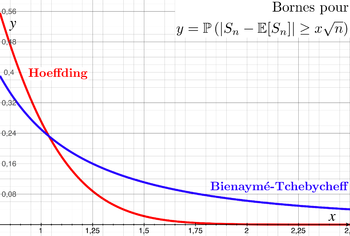
NOTE: Some people who are already familiar might ask why we use Hoeffding instead of something like chebyshev. Well, we kind of can, but it doesn’t guarantee a specific type of convergence, as we talked about above. Also, it’s not as tight as it possibly could be, so why would we use something that’s weaker? That means we may possibly need many, many more sample points than necessary to get to a specific confidence level of approximate correctness! Here’s an illustration:

Next Time

Next time, we talk about finite hypothesis classes, and how we can use hoeffding for a class of hypotheses using uniform bound. Here, we’ve only talked about a single hypothesis, which is not practical.

EDIT: Thanks to Andy for the typo fix :)