At my time at Airbnb, I’ve witnessed the development of the feature store effort on the machine learning infrastructure team. The project’s name is Zipline, and it has been presented at many conferences. As it’s one of the first open-sourced feature engineering platforms, I made sure to cover its implementation details in the query engine sections of the blog. The feature store problem is one of the most technically exciting problems for the data engineering space and many companies are trying to create their own solutions. I start by discussing the necessity of a feature store for ML applications and move on to talk about fundamental mathematical structures involved and some methods to solve the problem. The most important concepts are in the section about offline query engines, but the more novel ideas are in the section about the online query engines.
Table of Contents
- Table of Contents
- What is a Feature Store?
- Why do we need a feature store?
- Aggregation types
- Anatomy of the Temporal Join
- Query Engine (Offline)
- Other considerations
- Conference Talks
- Conclusion
What is a Feature Store?
A machine learning model does not typically use raw data as its features because of the following:
- Raw data often doesn’t show the bigger picture - it’s not a statistic representing a large quantity of data. Sometimes we may want to sum, average, etc the raw data for it to be useful.
- The raw data firehose and the sheer scale of it may negatively affect the training process(large aws costs for a single epoch), and require a much more complex online serving architecture to meet latency requirements.
- A lot of raw data is not useful - there could be nulls or missing information that require imputing on the fly.
- Raw data might not be in the form that the model can readily consume. (i.e. categorical variables are sometimes turned into one-hot encoding vectors)
Because of the reliance on processed data, there has been a growing demand for a component that can process and store these features. Feature stores are the solutions - they hold processed data that is used as input to machine learning models for inference, training, etc. Feature stores naturally can extend to support feature versioning, observability/monitoring tools and ad-hoc visualization tools in order to improve and understand the lineage and efficacy of features. It’s an abstract concept that can be implemented in many ways depending on the scale and specificity of your application. Generally, feature stores can deliver features to models in both online and offline settings (for both training and scoring), where in the online case latency is more important and in the offline case throughput is more important.
In the real world, data sources can come from anywhere - logs of applications (think Kibana log ingestion streams), daily database snapshots, pubsub messages (think Kafka messages), database commit logs and even data from other feature stores! It’s the feature store’s job to support and process these different data sources.
Why do we need a feature store?
Imagine you’re a data scientist or ML engineer for an e-commerce company, and you’re trying to develop a new machine learning model that detects whether the given user will purchase something in the current session. Usually the first step is to ask yourself “what features are causative to a user’s purchase patterns?”. Maybe after putting yourself in the shoes of the customer, you decided that if a person has spent a lot of money on this platform in the last 7 days, they will likely purchase something again in this session. You quickly come up with a couple more features and decide that XGBoost would be a good baseline for this classifier, and you can serve it in an online setting.
Now the first step is to see where in your data warehouse you can possibly find these features.
Let’s go through two example scenarios:
Scenario 1: Daily exports
After some digging, you found daily hive table exports in S3 with “dollars spent for the day” for every user. Great! Now you need to write a daily job to sum all past 7 days’ exports (excluding today’s since it hasn’t landed) for each user into a single table, so you can use that as your feature store for your model.
Scenario 2: Logs
After some digging, you found a raw data stream that contains the number of dollars spent for a user with a timestamp of the transaction. Great! You can create a table containing the total number of dollars spent for the day populated by the raw data stream, and export snapshots of it daily. Now you’re back at scenario 1.
But what if you want the past 7-days window to take into account the data received up until the very present? Then you would need to build something akin to a KV store that is updated every time a transaction occurs. Needless to say, this is a pretty complicated setup that wouldn’t be worth the marginal gain for most cases.
After doing this for a while, you quickly realize that collecting and cleaning data to create your features takes a long time and is repetitive. What if you can just declaratively express the data sources and the aggregations for your features and be done with it?
Requirements of a feature store
From the example above, you probably already have an idea of some requirements we need the feature store to support:
- Data recency: The daily exports scenario gives us features made from 1-day stale data, and that may not be acceptable for a system that’s sensitive to recent data or biases more towards intra-day events.
- Throughput: Table exports can be extremely large, and to enable newest features right after exports land, the feature store must be able to sustain high throughput to compute offline features.
- Online-offline consistency: The offline system that computes daily features and the online system that gives you the most up-to-date features must output the same result given the same inputs. We should expect identical setup if we were to bring an offline model to an online production environment.
- Feature repository: There are many features that can be shared among different models. This allows collaboration of multiple ML researchers and reduces duplication of effort.
- Monitoring system: If a feature recently changed anomalously, the researchers should be alerted in case their model isn’t trained to be robust under novel scenarios.
This is by no means an exhaustive list of requirements, but it should give you an idea of the challenges in designing such a distributed system aside from the typical consistency, availability, etc problems.
Aggregation types
It is sometimes necessary to aggregate features for them to be more useful. In the above example we used the sum of all purchases in the past 7 days. The key to understanding aggregation types is to focus on the word “sum” and “purchases”, i.e. an operator(in this case, the plus operator) working with a set of elements(in this case, numbers). In essence, we are combining raw data to create aggregations. Typical aggregation types belong in two categories, which we can rigorously define in mathematical terms. We’ll explain them briefly below.
Abelian Groups
A group is a set of elements $S$ (e.g. integers) with an operator $\cdot$ (e.g. addition) such that the follow properties hold:
- Identity
- Inverse
- Associativity
- Closure
An abelian group is one that contains this extra property:
- Commutativity (for Abelian groups only)
If we consider the aggregated statistic of “dollars spent in the past 7 days” by summing “dollars spent in a day” datapoints, we can show how each of these properties are important. In this case, we can model the set as all real numbers, and the binary operator as addition. Formally we can denote it as $(\mathbb{R}, +)$.
The identity of the group is 0, and it’s used to initialize a new user who just joined the platform and has spent no money on it. We want closure so that summing the past 7 days’ worth of transactions will still be a dollar amount. Associativity and commutativity are required so that the order of transactions or the way we group them for aggregation do not change our total sum.
So what is inverse used for? Well, it’s not actually required in the sense that we can still compute the total sum amount in the past 7 days without it. Instead, it is a powerful tool we can use to compute our statistics faster. Suppose we have a cumulative sum from when the user registered until times between then and today. It would be easy to compute the 7 days window by simply subtracting the cumulative sum until today with the cumulative sum until 7 days ago. Subtraction here is essentially adding the inverse element. We discuss this exact algorithm in more detail later in the blog. Note that if we chose our set as $\mathbb{R}_{\geq 0}$ then inverse would not apply and we would not have an abelian group. Instead we’ll have something called a commutative monoid.
Some useful examples of abelian group operators with sets as real numbers include addition/subtraction, multiplication/division, etc. With the set defined as $\mathbb{R} \times \mathbb{N}$, we can define averaging as an operator for this to be an abelian group as well.
How can average be represented as an abelian group?
Average can be expressed as an abelian group by using a 2-tuple in the form $(s, n)$, where $s \in \mathbb{R}, n \in \mathbb{N}$, where $s$ is the sum and $n$ is the count. When a value $s_t$ comes in and we want to update the average, we convert the value into the 2-tuple and add them:
\[(s, n) + (s_t, 1) = (s+s_t, n+1)\]As in, we increment the count by 1, and we add the value to the running sum. The inverse operation can be used to get an average of a time interval $[a, b]$ by the following:
\[(s_b, n_b) - (s_{a-1}, n_{a-1}) = (s_b-s_{a-1}, n_b-n_{a-1}) = (s_{[a,b]}, n_{[a,b]})\]The 2-tuple isn’t exactly an “average”, but contains enough information to retrieve an average, simply by $\frac{s}{n} \in \mathbb{R}$. We call the tuple an intermediate representation, or IR. Many aggregate types use IR’s that are bigger than a typical integer, and can go up to hundreds of bytes in practical applications. For reference, check out HyperLogLog, which is an approximate count aggregate which uses tunable IR sizes.
NOTE: We used +/- above to make the example less abstract, but in reality we’re adding by the inverse element when - is used above.
Commutative Monoids
Essentially, monoids are a superset of groups, in that they don’t have the restriction of inverses. A commutative monoid thus is just our abelian group without the inverse property. An example of a commutative monoid used in aggregation statistics is the max operator. Suppose we want to know the biggest daily transaction total for a user in the past 7 days. It is not always possible to figure out what the max is within the past 7 days from cumulative maxes because we’re dealing with a commutative monoid which doesn’t have an inverse.
Some useful examples of commutative monoid operators with sets as real numbers include max, min, median, etc.
Anatomy of the Temporal Join
When we’re defining features in the feature store, we typically ask the question “What is the <aggregation statistic> for <key> from <time A> to <time B>?”. This can be phrased by a join between the query and the raw data to create aggregated features. Semantically, the left side of the join is the query, the right side is the raw data, and the output is the aggregated features.
If we use the scenario 2 illustrated above as an example, we can have queries ask for “what is the total amount of money spent in some time range?”, with the raw events as purchase events with its corresponding dollar amount. The queries would look like:
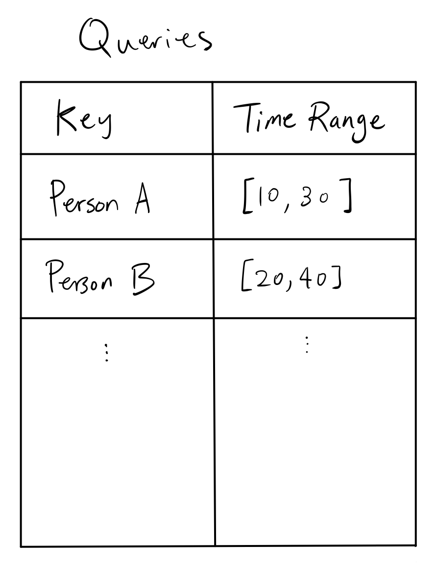 which is the left side of the join. Meanwhile, the raw events would look like:
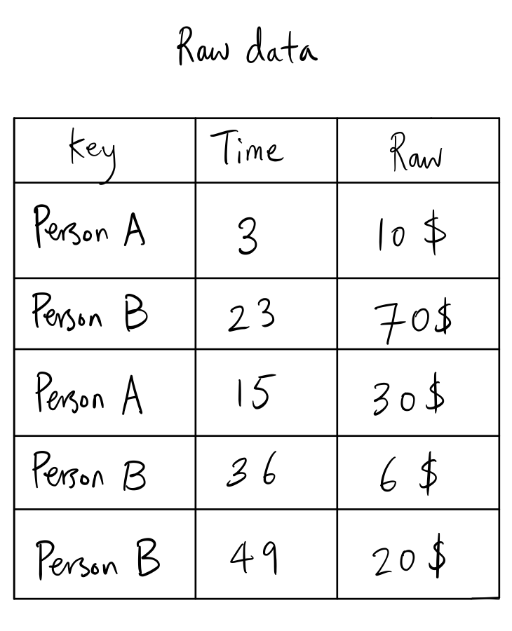
which is the right side of the join. The join looks like:
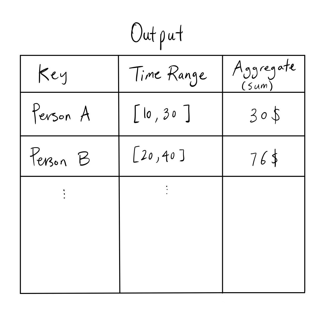
which is essentially a left join aggregated by name.
This looks like it can be done in SQL!
You’re right, we can answer the question above with a SQL setup:
CREATE TABLE IF NOT EXISTS `queries` (
  `id` int(6) unsigned NOT NULL,
  `name` varchar(100) NOT NULL,
  `starttime` int(3) NOT NULL,
  `endtime` int(3) NOT NULL,
  PRIMARY KEY (`id`)
);

INSERT INTO `queries` (`id`, `name`, `starttime`, `endtime`) VALUES
  ('1', 'A', 1, 5),
  ('2', 'B', 2, 3);

CREATE TABLE IF NOT EXISTS `events` (
  `id` int(6) unsigned NOT NULL,
  `name` varchar(100) NOT NULL,
  `time` int(3) NOT NULL,
  `value` int(3) NOT NULL,
  PRIMARY KEY (`id`)
);

INSERT INTO `events` (`id`, `name`, `time`, `value`) VALUES
  ('1', 'A', 3, 10),
  ('2', 'B', 23, 70),
  ('3', 'A', 15, 30),
  ('4', 'B', 36, 6),
  ('5', 'B', 49, 20);

SELECT queries.name, queries.starttime, queries.endtime, SUM(events.value) FROM queries LEFT JOIN events ON queries.name = events.name
  AND queries.starttime <= events.time AND events.time <= queries.endtime
  GROUP BY queries.name;
The problem statement, formulated in SQL, only accounts for the offline application for the feature store and not the online applications. We discuss efficient ways to solve the offline feature store below, and try to unify the solution in the online case.
In the meantime, if you’re comfortable thinking about the problem setup as joining tables in relational databases, it’s a great analogy to use for the rest of the blog.
Query Engine (Offline)
As we discussed before, abelian groups and commutative monoids should be considered differently because of the missing inverse property. The reason is because the optimal algorithm for ranged aggregate queries are different. Intuitively, the more restrictions and structure, the more optimal the algorithm, and we’ll discuss that below. Before we do that, let’s define some variables in our problem:
$N \in \mathbb{N}$ is the number of events containing raw data.
$M \in \mathbb{N}$ is the number of queries the user makes with arbitrary range.
We are considering an offline algorithm in which the queries and events will not mutate.
Array-based Algorithms
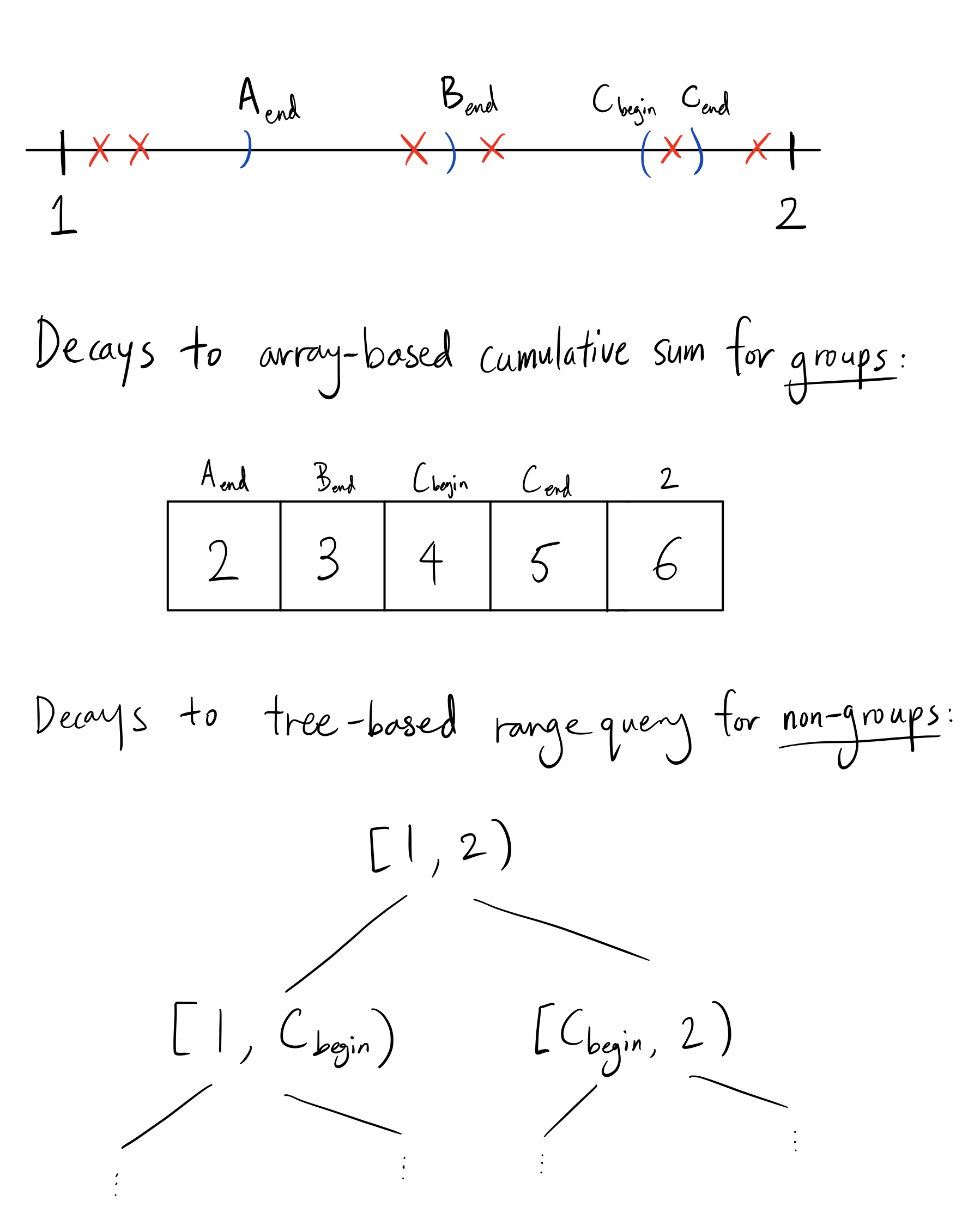
Suppose we use the abelian group $(\mathbb{R}, +)$ for example, and we have $M$ queries and $N$ events. Suppose we have a discretized timestamp (by minutes, for example), then denote $G$ as the number of bins we can put timestamps into. We can have the cumulative sum from some starting time until now with the aggregates we’re interested in. Since inverses exist, we only need to find two cumulative sums and find the difference as the range query:
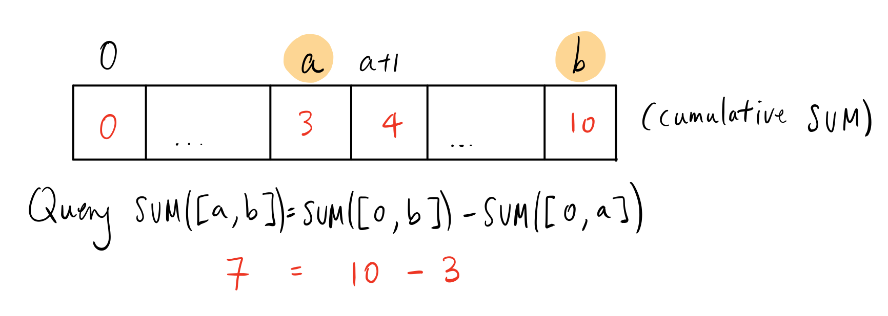
This algorithm is fast because it uses the fact that inverses exist in abelian groups. If $G$ is small, this array can fit in memory. To populate all events, it takes $O(max(N,G))$, since we’ll need to create a cumulative sum array after putting $N$ elements into the array bins. Each query is $O(1)$, or $O(M)$ in total. Thus, the overall runtime is $O(max(N,G) + M)$. The space complexity would be $O(G)$ since there are $G$ elements in the array.
It is important to note that we are sacrificing precision for speed in the tradeoff for $G$. It’s a tunable parameter, which adds to the complexity of this algorithm.
Tree-based Algorithms
Suppose we have a commutative monoid(note that abelian groups are also commutative monoids), then we can use a segment tree for range queries. Given the number of bins for timestamps $G$ as before, we can construct the segment tree with all events in $O(Nlog(G))$ time and query M times for $O(Mlog(G))$ time. In total, we have $O((N+M) log(G))$ for runtime and $O(G)$ for space.
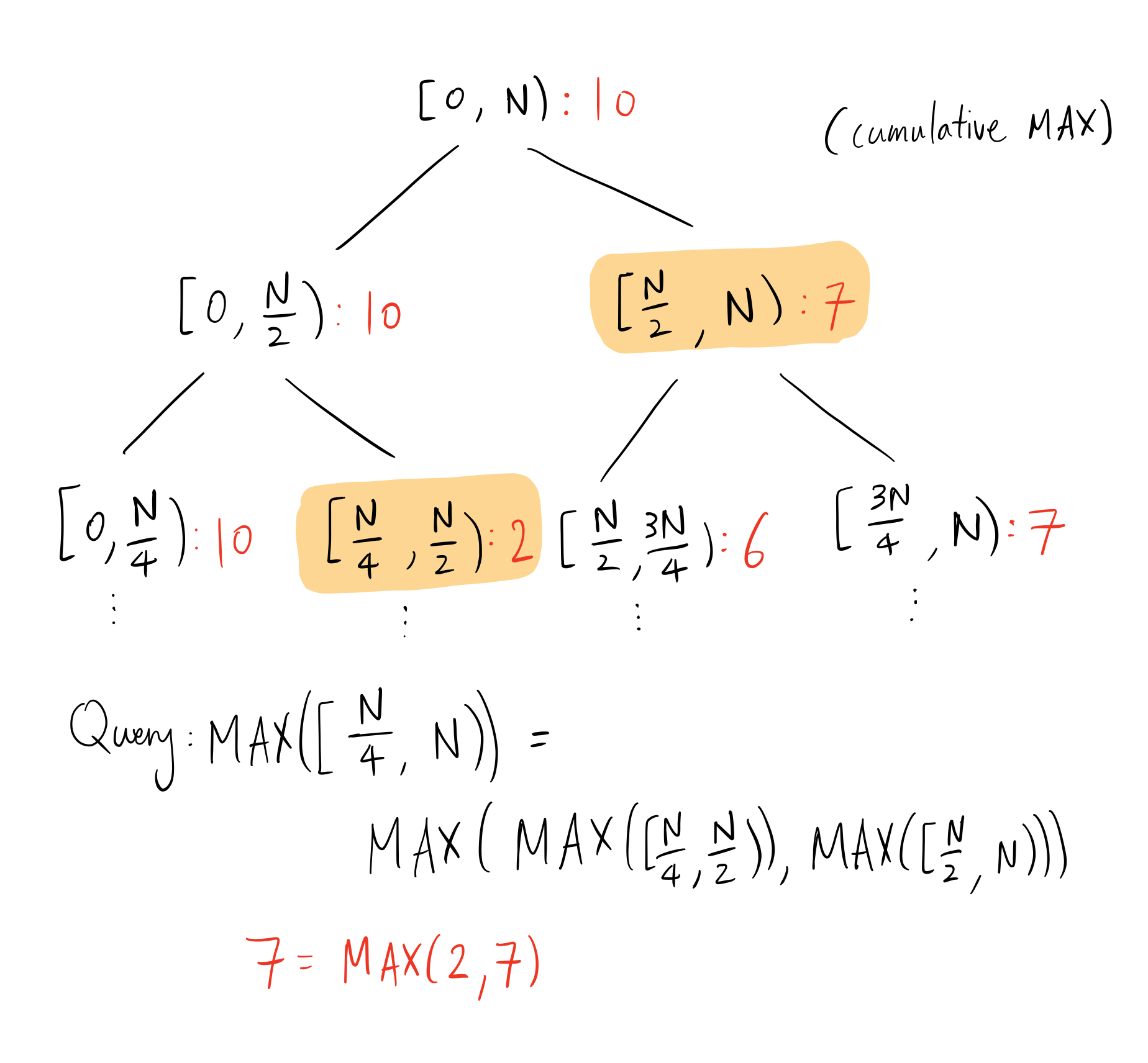
Here, N is the number of discretized timestamps - not to be confused with N as the number of events. This is a very typical use-case of segment trees, and so typical optimizations like lazy propagation play important practical roles to prevent redundant updates. The segment tree displayed in the diagram above is binary but does not need to be - increasing the branching factor decreases the depth of the tree but adds overhead to queries. Note that we can use fenwick trees for the same purpose. To keep this blog fairly self-contained, we only discuss segment trees.
Alternative Segment Tree Representation
An observation we should make is that we don’t care about the order of elements on the time scale as long as we know which queries should take it into account(this implies that queries are fixed). One optimization we can make to the segment tree is to have leaves represent the spaces between endpoints of intervals in the query rather than the integral timestamps:
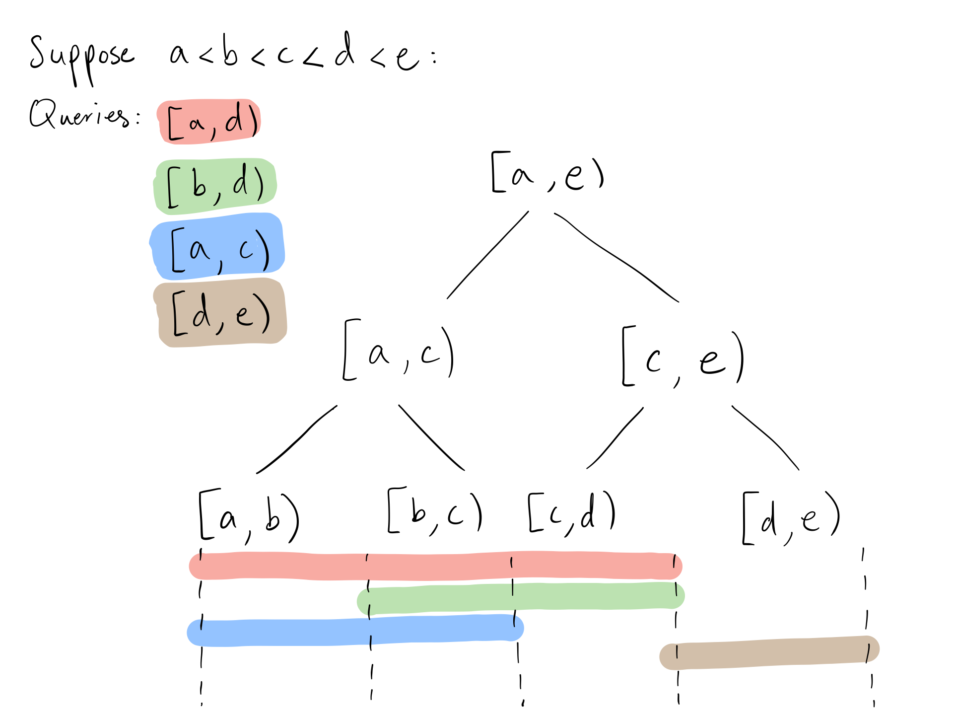
For any $M$ number of queries, we have at most $2M$ leaves in this segment tree, thus insertion and query will take $O(Mlog(M))$. The total runtime is $O((N+M)log(M))$, which is independent of $G$. The space complexity is now $O(M)$.
Skiplist-based Algorithms
Skiplists are data structures which allow access of a particular element in $O(logN)$ time, by creating hopping links in a linkedlist that requires logarithmic traversals to get to any point in the list using exponentially increasing sizes of hops. In the same way, we can decompose any query into a(roughly) logarithmic number of queries, each which can be performed in $O(1)$ time. Skiplists are commonly used in the index engines for relational databases and K/V stores, and Zipline is currently using the skiplist approach for both the online and offline use cases. As a result, there are more empirical results and recommendations I’ve provided for this algorithm.
Before we accept events, we tile the timeline into window sizes, each window size geometrically larger than the previous (refer to the below diagram for an example). For any event, it would need to update a single window in each granularity (there are logarithmic number of different window sizes). This algorithm works for any commutative monoids. In practice, the precision is limited to some granularity to reduce memory pressure, e.g. using seconds as the smallest window size, when events come in at the millisecond scale.
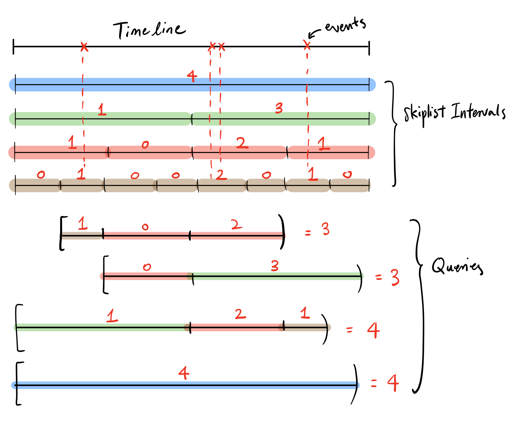
The number of windows we need to query for any given range is logarithmic as we can see in the example above. If many queries have large overlaps, the windows’ results can be cached for quick re-access.
We take care of any query requiring more precise windows with a concept in Zipline called accumulations. This part isn’t necessary for understanding the skiplist implementation if you don’t care about fine-grained precision, i.e. if we’re only dealing with queries with integral precision in the example above.
So what are accumulations?
Accumulations in Zipline are query-specific intervals between the smallest granularity and the endpoint, which are used to construct the “tails’’ of intervals that do not fit nicely into the smallest granularity. One good thing about accumulations is that it works well with “infinite precision” ranges which can include irrational, trascendental, or repeating decimals.
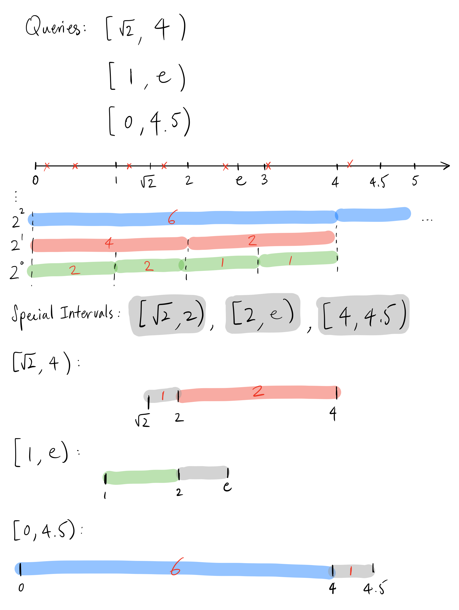
As we can see in the diagram above, the accumulations are used to compute the remainders in the start and end of intervals.
Without accumulations, the overall algorithm is $O((M+N) log(G))$ time complexity and $O(G)$ space complexity. With accumulations, we must deal with the case that there are multiple interval endpoints that lie between the smallest granularity. In the case that all intervals lie within the same accumulation, the case degenerates into the above segment tree algorithm in the alternative form.
So the basic idea of accumulations is to delegate the smaller remainder interval aggregate calculation to a different algorithm, one that can handle arbitrary precision on the start and end times of intervals.
Overall, the worst case is a logarithmic number of skip list queries with a logarithmic range query in the accumulation. This amounts to $O((M+N) (log(G) + log(M)))$ for time complexity and $O(G+M)$ for space complexity.
NOTE: The skiplist approach has many similarities with the tree approach, and one can think of the two as equivalent.
Theoretical Optimization
In Chazelle’s paper here, the algorithm aims to solve a generalized version of this problem. Specifically, given a d-dimension rectangular query $q = [a_1,b_1] \times … \times [a_d, b_d]$, compute partial sums of data points in the array $A$.
\[\sum_{(k_1,...,k_d)\in q} A[k_1,...,k_d]\]In our case, we are only querying based off of time, which is a one-dimensional query. In our case, we can rephrase it as:
\[\sum_{t \in q} A[t]\]Where $A[t]$ is the unaggregated raw data associated with the event at time $t$. The result is that with $N$ events and $M$ queries, it is possible to retrieve the aggregates in $O(M*\alpha(M,N))$, where $\alpha$ is the inverse Ackermann function. The partial sum block sizes are dictated by the growth function $R(t,k)$, where $t$ is the runtime calculated in the number of sums required for any range query, and $kM$ is the array space required for allocation. The two-parameter growth function is defined recursively in a format similar to the Ackermann function.
\[R(1,k) = 1 \quad \forall k \geq 1 \\ R(t, 1) = 4 \quad \forall t > 1 \\ R(t, k) = R(t, k-3)R(t-2, R(t, k-3)) \quad \text{otherwise}\]The above is only defined for $k = 1+3n \forall n \in \mathbb{N}$ and $t = 1 + 2n \forall n \in \mathbb{N}$, but we use the growth function to upper-bound the scheme required to build the partial sum blocks. The scheme finds the smallest $(t,k)$ pair with priority for $t$ to be minimized such that it is greater than the time range, divided into $R(t, k-3)$ sized partial sum chunks, and the process repeats recursively.
In reality, this is similar to our algorithm but generalized to multidimensional rectangular queries and using a different step size for partial aggregates. We create partial sum windows that are exponentially growing, yielding logarithmic runtime complexity. The result above is using windows growing roughly at the rate of the Ackermann function, and thus it yields inverse Ackermann runtime complexity. In practice, no software scale has come close to requiring inverse Ackermann, and we can use the first few levels of Ackermann function block sizes to yield super logarithmic time complexity for our use case. Even then, it may be overkill and introduce more overhead than expected.
Other considerations
Relaxing requirements for optimizations
Windowed vs. Non-Windowed
We describe a set of queries to be “windowed” if each query can have an arbitrary beginning time, and “non-windowed” if each query in the set has a fixed beginning time and an arbitrary end time. Non-windowed queries are common - and they often ask questions about the running state of a user, like “how many items did this person purchase on our platform until some date?”. If we fix the beginning time for all queries, there would be small optimizations we can make to the existing algorithms.
One such optimization would be to take advantage of the fact that we can answer all the queries in a batch setting offline. We can construct a partial aggregate separated by end times of the queries in an array. To insert an event, we perform binary search on the boundary timelines which takes $O(log(M))$. Finally, we perform an accumulation of the partial sums in-place:
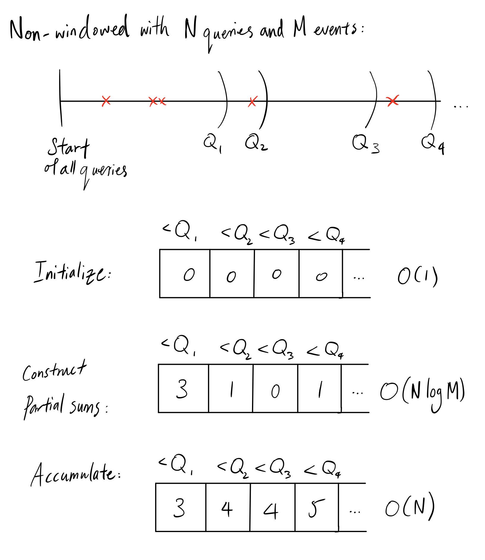
To insert a particular event into an optimized segment tree(separated by endpoints of queries, not time), previously we had to search in $O(log(M))$ time and update in $O(log(M))$ time. Now, we only need to construct partial sums which only requires a single update, with an accumulation afterwards.
Although it’s not an asymptotic upgrade in runtime(both require logarithmic time in search), in systems like Zipline, this has shown to improve practical performance significantly.
Online equivalents
In an online system, the problem becomes invariably harder. In the offline setting, we mostly cared about correctness and performance in terms of throughput. In the online case, we additionally care about performance in terms of latency. In the case we want to unify online and offline systems into a single abstraction, we also care about consistency, or as we previously called it: online-offline consistency. The consistency guarantee is that the online and offline results must be identical given the same inputs. We obviously wish to have all of these properties but under specific load and conditions, we may need to sacrifice one or more of these requirements.
Tree-based Algorithms
As the online system stays online longer, the bigger the segment tree becomes. Adding leaf nodes to existing segment trees to increase the range is usually not a good idea. Instead, the strategy is to create a new root node which is twice the range of the current tree, and attach the current root to the left. In an online setting, the allocation of a new root and a new subtree denoting events in the future time frame can be done in the background when a time threshold is met.
Because we don’t know when the queries will come, we cannot apply the optimization to the segment tree to only consider the query windows as ranges. Therefore, we must opt for a segment tree with ranges on time intervals. To have a fully binary segment tree, storage would be inefficient since there are $10^{10}$ milliseconds in a year. Although it may be able to store the segment tree completely in high memory instances, we can do better. An observation is that we don’t need the full segment tree to be specified. The tree itself can be relatively sparse, and only contain a leaf at an event’s timestamp. The absence of a tree node signifies $0$ events within that range. Below is an illustration of that:
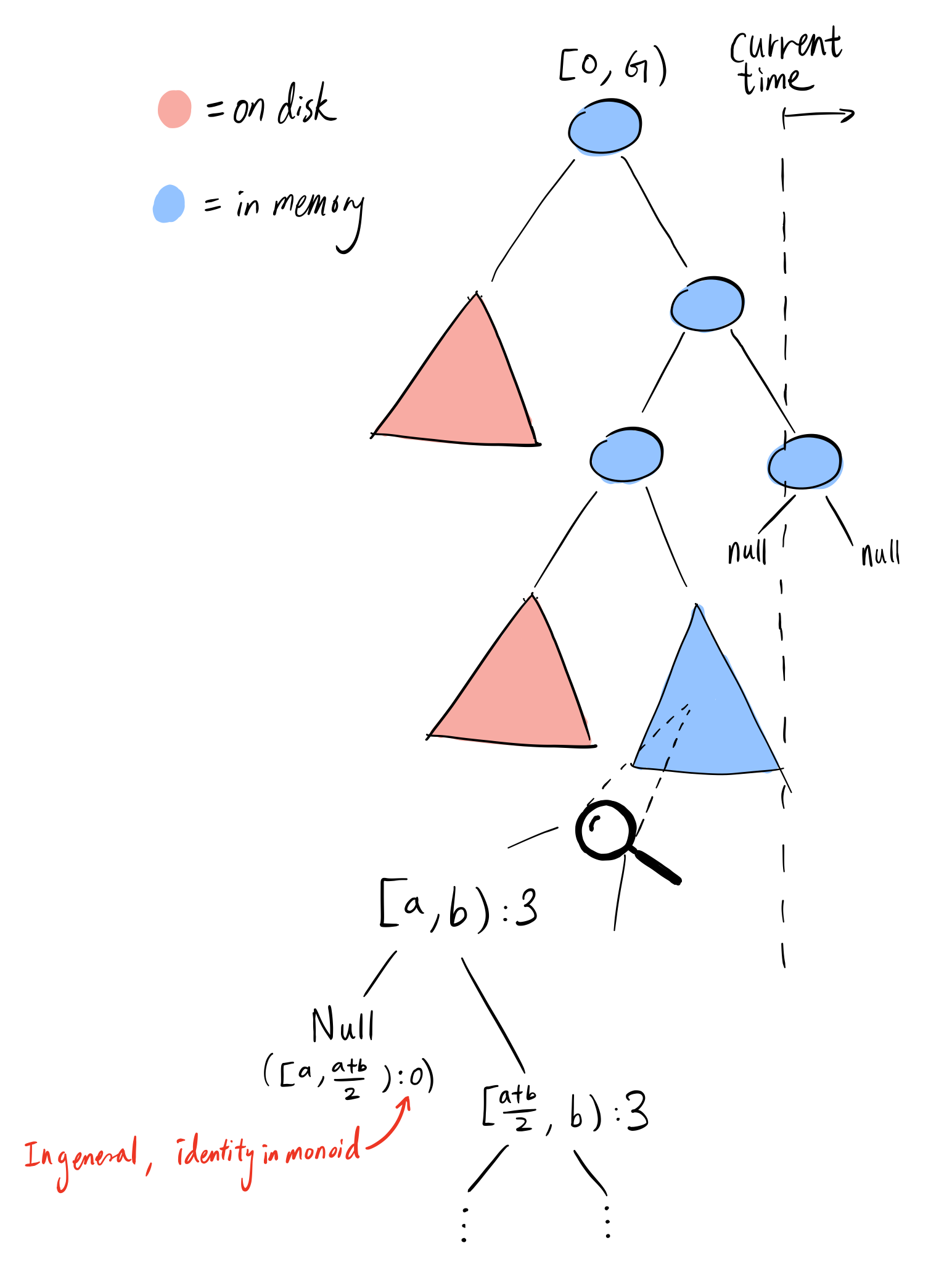
Then, at any point in time the tree will have at $max(G, N)$ leaves. If we’re dealing on the 1-year max range scale and a binary segment tree, then every leaf(which associates with an event) would require on the order of $\sim30$ traversals down the tree. It is likely that with a high number of events, the tree would not be sparse, and the traversals will lead to cache misses. If ultra low-latency was not a primary concern, this design would be very efficient.
Suppose we have a tree too big to fit in memory, e.g. the time scale expands past a year and the tree needs to double in size, we can assume the left subtrees will not likely be accessed nor updated often in an online setting. For updates, Incoming stream data may be late by at most a few minutes to hours, and for queries, the features are usually computed with recent aggregates. To reduce the memory pressure, we can compress the left subtree(which could be very sparse) into a disk-friendly segment tree which can then be queried later in the offline case.
There are many types of distributed segment trees out there, like ones based off of distributed hash tables like Shen et. al.. These implementations are generic and don’t optimize for access patterns that zipline does in an online setting. We keep the front of the tree in memory to make the majority of queries efficient, meanwhile distributed segment trees are not specifically built for the front-biased queries.
A Case Study
Suppose we have an online system running with the above design for 1 year, and events are ingested at a rate of 100/sec. Furthermore, we assume each event’s timestamp is unique, with granularity up to the millisecond scale. We’re interested in the time it takes to query for an aggregate from 10 days($\sim 2^{30}$ milliseconds) ago until now. In total, we have $100 * (60 * 60 * 24 * 365) \approx 3 * 10^9$ events stored, or number of leaves in our segment tree. Suppose we perform the storage optimization so that only 1 month of aggregates are stored in memory, and the rest is on disk in an optimized format. Then we have $\sim 3 * 10^8$ events in memory and $\sim2.7 * 10^9$ on disk. If we represent each node in the segment tree with $128$ bytes (which for most cases is reasonable except for topK, HyperLogLog, etc), then we’ve only used on the order of $\sim3 * 10^{10}$ bytes, or $\sim 30$GBs, which is reasonable for a typical server machines with $\geq 100$ GB of RAM (a full binary segment tree only doubles the number of nodes, ours being sparse is a slightly higher constant factor overhead). We also have roughly $\sim 244$GB times a constant factor(to create an in-disk segment tree) worth of events stored in block storage, typically on SSD’s.
Given a query of 10 days, the entire query can be done in memory. Since 10 days is equal to $\sim 2^{30}$ milliseconds, the subtree’s depth is at most 30. Suppose in the worst case, we query for $log(2^{30})=30$ nodes in our data structure for the range query, each of which is descending by 1 level. In this worst case of a binary segment tree, we require $2*logM$ nodes to traverse, which in this case is 60. Equivalently, it is the number of memory locations we need to access, all relatively far away from each other. Suppose we don’t run into any page faults, then the worst case scenario is 60 local DRAM accesses, which is roughly on the scale of $100ns$ each. In total, the query would have taken 6 microseconds just for the tree traversal itself. However, a single hop even within the same AWS VPC is on the order of milliseconds as discussed here, so it is fairly negligible in the typical service oriented architecture that many companies are converging on. Unless the feature store needs to be an embedded application(in which case we do not need a network hop) and we are dealing with sub-microsecond latency requirements, this approach operates well within requirements.
Skiplist-based Algorithms
The reason we’ve mentioned the skiplist based algorithm above even though it performs slightly worse than the segment tree approach is because a segment tree is fixed to a specific interval. The skiplist alternative can be easily fitted for online feature serving because we can simply add new windows for aggregates. The simplest generalization of skiplist to the online equivalent rests on the assumption that the immediate features must be taken into account, but the window size could be slightly off. We will begin by rounding the start times of queries down to fit the biggest sub-intervals, then increasingly add smaller intervals until we reach the cumulation. Below is a diagram for this:
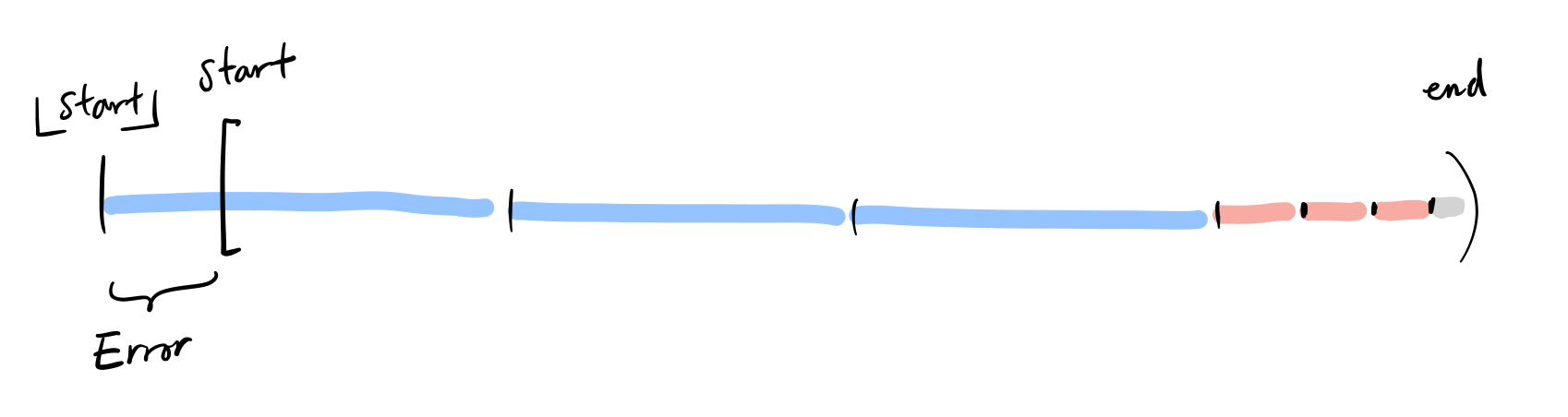
If we define the ratio of error interval with the original interval, we can prove that for any window size that grows exponentially(with integral growth factor > 1), the range of error can be anywhere in $[0, 1)$. Having a near-100% error ratio is bad for various reasons, but there is a way to trade off constant overhead for a lower error margin. We can define the max size window used for ranges of intervals to decrease the error margin. For example, if we have doubling window sizes, and we have an interval of length 9, then by default we’d use 2 windows of size 8, as it’s the biggest interval we used. However, that is almost a 100% error ratio(⅞), and we can decrease this by forcing intervals of length 8-16 to use window sizes that only go up to 4, not 8. In this case, we’d use 3 windows of size 4, leaving the error ratio to be closer to 50%(⅜). In the doubling window case, we can get the error to $1/ 2^k$ if we increase our expected number of windows by $2^k$ times. Similar arguments hold for different exponentially growing window sizes. In Zipline, these restrictions on max window sizes are called “hops”.
Note that the above greedy approach is the same as the coin change greedy algorithm, which requires the coin system to be canonical according to Pearson et. al. A coin system being canonical is defined as a coin system where the greedy solution for arbitrary change(picking the largest denominations first) is always optimal. To verify our window sizes are indeed canonical, the algorithm presented by Pearson et. al is $O(N^3)$, where $N$ is the number of different coin denominations.
In addition, in the real world, performance may come second as compared to the concept of online-offline consistency. To be consistent, any range queries performed in the offline setting must also report the same result in the online setting. This is because model prototyping, training and backtesting is often done in an offline setting. To feed a model slightly different input could lead to large perturbations in performance metrics. In the world of general software engineering, consistency is often chosen in the tradeoff between consistency and performance. Since Zipline is implemented using the skiplist approach and requires consistency, the offline equivalent used in Zipline returns an approximation of the range query by rounding the start date to ensure the online and offline algorithms are identical.
Theoretically speaking, although the skiplist approach sacrifices correctness slightly, it is faster in practice since it would theoretically incur less cache misses(all of the partial sums of a particular window size are contiguous in memory) and is simpler to implement. For large aggregates, such as hyperloglog and topK, this architecture can handle large queries better than the segment tree approach due to sequential reads on disk for large aggregates.
Conference Talks
Of course, this blog focused on the engine portion of the whole process, but did not cover some crucial details such as the DSL(domain specific language) for the feature store queries, the integration of feature store with existing data sources in a typical company, implementation using Spark, etc. These topics are covered in my coworker’s talks shown below, specifically for Airbnb’s Zipline project:
Nikhil at Strange Loop
Varant and Evgeny at Spark Summit
Conclusion
Feature stores are an upcoming technology that enables accelerated development of robust and powerful machine learning applications. Large parts of boilerplate offline model training can be abstracted away, and data scientists can now use point-in-time correct features in an online setting. For Airbnb, this was a humongous leap in efficacy of machine learning models, especially within the fraud detection organization. As with any adequately complicated piece of infrastructure, there will always be theoretical and practical improvements in the future that this blog fails to cover. I hope to update this entry when I’m notified of future developments!
Disclaimer: The opinions expressed in this post are my own and not necessarily those of my employer.