I haven’t been writing blogposts as often as I’d like to, but mostly for the reason that I don’t have a lot of time to goof around. Now that I have some free time, Tiff reminded me that I should write something. I will write more about this subject when I have the chance.
What is Computability Theory?
Computability theory is a branch of mathematics that attempts to analyze and categorize problems into ones that can be decideable or computable under some given restrained resources. These resources are fairly applicable to real life scenarios, i.e. memory or time. I’ve had the privilege of learning from Yiannis N. Moschovakis and Amit Sahai, who are both very knowledgeable in this field. Here I attempt to condense some of the material into digestible readings for those who want to get a brief introduction. It does require a bit of mathematical background as I will be assuming that you know basic proofs by induction and some notation.
Recursion and Primitive Recursive Functions
It is intuitive enough that in order to find out what our computers can do, we start with induction and recursion. For loops and otherwise complicated programs have some type of implicit recursion. It turns out that the principle of mathematical induction and the basic recursion lemma are almost synonymous (one can prove induction given recursion, and vice versa).
The basic recursion lemma(a result of Kleene’s second recursion theorem) is stated as follows: For all sets $X,W$, and any given functions $g:X\to W, h:W \times \mathbb{N} \times X \to W$, there exists one unique function $f:\mathbb{N} \times X \to W$ such that:
\[f(0,x) = g(x), \\ f(n+1,x) = h(f(n,x), n, x)\]Basically, $f$ can be recursively defined by some “generating function” $h$ and some “base function” $g$. All of the interesting functions we can compute on our computers are recursive in nature.
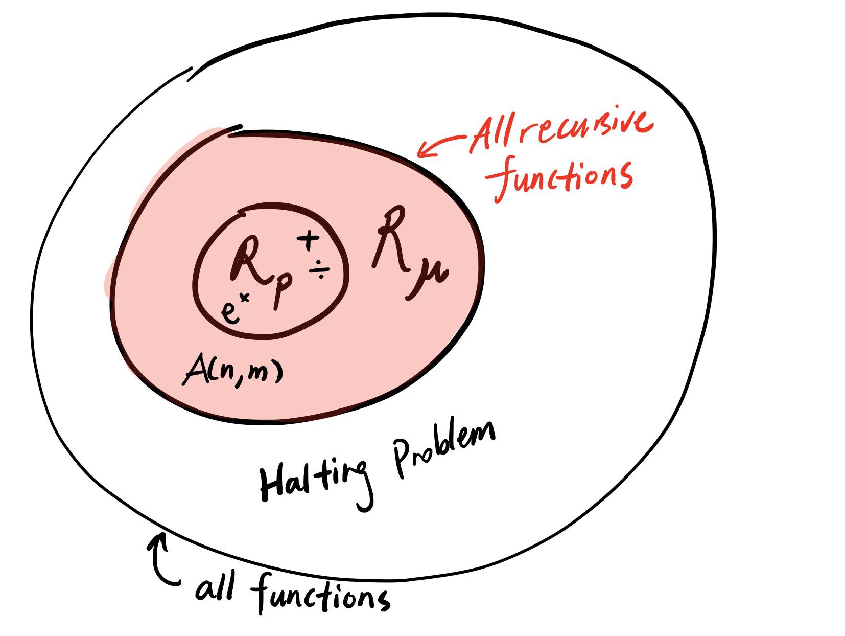
There is a specific class of recursive functions, called primitive recursive, denoted as $\mathcal{R}_p$. Roughly speaking, it is the set of functions that are defined by:
- Constant functions are in $\mathcal{R}_p, C^n_q(x_1,…,x_n) = q$
- The projection functions are in $\mathcal{R}_p, P^n_i(x_1,…,x_i,…,x_n) = x_i$.
- The successor functions are in $\mathcal{R}_p, S(x) = x + 1$.
- Any composition of (1-3) are also in the set.
- If $g, h \in \mathcal{R}_p$, and $f$ is defined as: \(f(0,x) = g(x), \\ f(y+1, x) = h(f(y,x),y,x)\), then $f \in \mathcal{R}_p$.
We can build addition, multiplication, exponentiation, if-statements, loops, etc from this set of functions. Most of the functions we use in computer science can be expressed as some $f \in \mathcal{R}_p$.
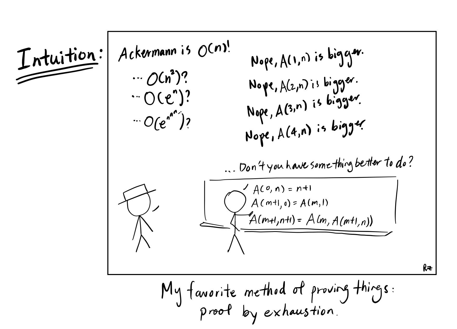
An example of a recursive function that is not primitively recursive is the Ackermann function, which we will discuss in detail later:
\[A(0,x) = x + 1, \\ A(n+1, 0) = A(n,1), \\ A(n+1, x+1) = A(n, A(n+1, x))\]It is not clear at first that $A$ has a unique solution; the proof is done via double induction. We first suppose there exists $f, g$ which are solutions to $A$ for some inductively increasing subdomain, and then we show that they must be equal.
- Sub-induction: $A(0, 0) = 1$. Then $f(0,0) = g(0,0) = 1$. And it is clear that $\forall x, f(0,x+1) = g(0,x+1) = x+2$, so they are unique.
- Base: Suppose $\forall x, A(n, x)$ has a unique solution $\implies A(n+1, 0)$ unique as well. This is true since $A(n+1, 0) = A(n, 1)$, which we know is unique, so $f(n+1,0) = g(n+1,0) = f(n,1)$.
- Inductive: Suppose $\forall n \geq 1, \forall x, A(n-1,x)$ has a unique solution, as well as $A(n, k)$ by the inductive hypothesis. Then, $A(n, k+1) = A(n, A(n+1, k)) = f(n, f(n+1, k)) = g(n, g(n+1, k))$ must be unique.
Why Ackermann isn’t Primitive Recursive
Intuitively, if you fix Ackermann’s sections, $A_n(x) := A(n,x)$, you can inspect the value to see that it is growing extremely quickly. One can think of the growth like the following: the 0-th section is successor, 1st section is addition, 2nd section is multiplication, 3rd section is exponentiation, 4th section is hyperexponentiation, etc. The rate of growth from every section to the next is growing so fast that you can’t really use big $O$ bound using any common functions.
In order to prove $A \not\in \mathcal{R}_p$, we take an arbitrary function $f \in R_p$, and show that $f < A_n$ for some $n \in \mathbb{N}$. This rough sketch on growth shows that every $f$ that is primitive recursive is bounded by $A$, so $A$ cannot be in $\mathcal{R}_p$. I opted for this to be easier to digest so the trivial claims I make without proof are marked with $*$ . One claim we will make is the following:
The nested Ackerman call is bounded by itself, i.e. $A_n(A_n(x)) < A_{n+2}(x)$.
-
Sub-induction: $A_0(A_0(x)) = x + 2 < A_2(x) =^* 2x+3 \forall x \in \mathbb{N}$. A simple induction proof shows the latter equality.
-
Base: Suppose $A_n(A_n(x)) < A_{n+2}(x)$. Then:
\[A_{n+3}(0) \\ = A_{n+2}(1) \\ = A_{n+1}(A_{n+2}(0)) \\ = A_{n+1}(A_{n+1}(1)) > A_{n+1}(A_{n+1}(0))\] -
Induction: Suppose $A_n(A_n(x)) < A_{n+2}(x) \forall x$ and $A_{n+1}(A_{n+1}(k)) < A_{n+3}(k)$, then $A_{n+1}(A_{n+1}(k+1)) < A_{n+3}(k+1)$ since
\[A_{n+3}(k+1) = A_{n+2}(A_{n+3}(k)) \\ > A_{n+2}(A_{n+1}(A_{n+1}(k))) \\ > A_{n+2}(A_n(A_{n+1}(k))) \\ = A_{n+2}(A_{n+1}(k+1)) >^* A_{n+1}(A_{n+1}(k+1))\]
This result will be useful for later.
To start off, our inductive hypothesis will be that for any $f \in R_p$, $f(x_1,…,x_m) < A_n(max\{x_1,…,x_m\}$ for some $n \in \mathbb{N}$.
If $f$ is the successor function, then $f(x) = A_0(x) <^* A_1(x)$. If $f$ is the constant function that returns $q \in \mathbb{N}$, then $f(x_1,…,x_m) = q <^* A_q(0) \leq A_q(max\{x_1,…,x_m\})$. If $f$ is the projection function, then $f(x_1,…,x_n) = x_i \leq A_0(max \{x_1,…,x_n\})$.
We have established the base cases. For more interesting functions, if $f$ is a composition of functions, i.e. \(f(x1,...,x_n) = h(g_1(x_1,...,x_m),...,g_m(x_1,...,x_m))\), and by inductive hypothesis we can assume $g_1,…,g_m,h$ are bounded by some $A_k(max\{x_1,…,x_n\})$ (just take the max $k$ for all of the functions). Then the composition is bounded by $A_k(A_k(x)) < A_{k+2}(x)$, using the claim above.
Finally, for some $f(n,\bar{x})$ defined like (5) in the primitive recursive section above, it is slightly trickier. By the inductive hypothesis, we can assume $g, h < A_{k-1}$. Then we claim the following: $f(n,\bar{x}) < A_k(n+\{\bar{x}\}) $. We denote $x := max\{\bar{x}\}$ for the proof.
- Base: $f(0,\bar{x}) = g(\bar{x}) < A_{k-1}(x) < A_k(x) = A_k(x+0)$ as given.
- Induction: Suppose $f(n,\bar{x}) < A_k(x+n)$ . Then $f(n+1, \bar{x}) = h(f(n,\bar{x}), \bar{x}, n) < h(A_k(x+n), \bar{x}, n)$. Since $A_k(x+n) > x+n \forall k \in \mathbb{N}$, we see that the growth of arguments in $h$ is dominated by $A_k(x+n)$, so $h(A_k(x+n), \bar{x}, n)\leq A_{k-1}(A_k(x+n)) = A_k(x+n+1)$.
Take $z = max\{x, n\} = max\{x_1,…,x_m,n\}$, then $f(n,\bar{x}) < A_k(x+n) \leq A_k(2z) < A_k(2z+1) = A_k(A_2(z-1)) < A_k(A_{k+1}(z-1)) = A_{k+1}(z)$. And so we have that $f(n,\bar{x})$ is bounded by another Ackerman function section.
The above is a sufficient proof to show that $f \in \mathcal{R}_p \implies \exists k \in \mathbb{N}, f < A_k$. Now, suppose $A$ is primitive recursive, then that means $h(n, x) = S(A(n,x)) = A(n,x) + 1$ must also be primitive recursive. Then there must exist some $k$ such that $h < A_k$, which is absurd and concludes our proof.
It seems intuitive that if something grows faster than all of the primitive recursive functions, then it cannot be primitive recursive. It grows so fast that at $A(4,2)$, it returns an integer with 19729 digits.
Quick Aside: \(\mu\)-recursiveness
Then what can we characterize the Ackermann function as? We can, technically, write a (long) while loop and search for the next value of Ackermann. This (albeit neverending) while loop is technically a \(\mu\) operator, which gives us the least solution that satisfies some conditions. This is vague, and I will expand on it on the next blogpost. We call any function that can be written with arbitrary while loops and primitive recursive building blocks as \(\mu\)-recursive, and Ackermann is one of such functions.
What else is out there?
Though Ackermann is not something we can practically compute for high digits, it is still in theory, “computable” by a recursive program. Then, I guess that begs the question - What can’t our computers compute? The results we will explore don’t only influence computer science, but answers* questions about philosophy, abstract mathematics, and many other things in our world.
*: By answer, I don’t mean that answer to the universe and to life is 42, but rather, a concrete answer detailing why “there’s no way we will ever find out”.