Table of Contents
- Table of Contents
- Recap of Ackermann and $\mu$-recursive
- Partial Algebras
- Normal Form and Enumeration Theorem
- The Halting Problem
- Why Do You Care?
Recap of Ackermann and $\mu$-recursive
Recall that our previous result was that $A(n,x)$, the Ackermann function, is not primitive recursive, which means it’s not in $\mathcal{R}_p$, but it is a recursive function. It turns out that it is in the class $\mu$-recursive functions. This $\mu$ means the “least” operator, and $\mathcal{R}_\mu$ is the set of functions that not only holds all properties of primitive recursive functions but also closed under composition of the $\mu$ operator, which is defined as the following: \((\mu i\geq y)R(i,\vec{x}) = \text{least i} \geq y \text{, such that } R(i,\vec{x}) \text{ holds.}\) where $R(i, \vec{x})$ is a relation. This means that for all $j < i$, $\mathcal{X}_R(i, \vec{x})$ the characteristic function of $R$, is divergent or is 0. We will later see that $\mu$-recursive is equivalent to the set of all possible recursive functions, and we will finally relate it to the halting problem.
Partial Algebras
When I say “algebra”, I don’t mean “solve for $x$ in the equation $3x + 2 = 0$”. It is something much more general - it is the study of mathematical symbols and their corresponding rules. When we talk about the numbers $0,1,2,…$, and the functions $+, -, \times, \div$, we are thinking in a specific algebra. The algebra that we are thinking of is defined by:
\[\textbf{Q}_1 = (\mathbb{Q}, 0, 1, +, -, \times, \div) \qquad \text{(0, 1 can be omitted, but kept traditionally)}\]By definition, all functions in this algebra must be a mapping $: \mathbb{Q} \to \mathbb{Q}$. The operators $+, -, \times$ can be applied to any number in $\mathbb{Q}$. However, $\div$ cannot. This is an example of a partial function, as in only part of the domain of $\div$ can be evaluated. We denote $\div : \mathbb{Q} \rightharpoonup \mathbb{Q}$. Our normal functions that maps every element in its domain to some value is called a total function in this context. A partial algebra is just an algebra that allows us to have partial functions. We denote undefined-ness as divergence with $\uparrow$, for example $\div(x,0) = \uparrow$. In addition to functions, and numbers, we also have variables in algebra. We can have any arbitrary $v_1,v_2,…$ as symbols in our expressions. To make equations, we have $=$ as a valid symbol as well. To allow branching conditionals, we have $\text{if, then, else}$ as symbols. To allow for multiple symbols in a function call, we have $,$ to separate arguments.
Examples:
- $\div\text{if}3))$
- $3,23\times$
- $\text{if }(\frac{3}{2}=0)\text{ then }23 \text{ else }2$
Intuitively, the first two don’t really “evaluate” to anything, and the last one evaluates to $2$.
In computer science, we can usually express most of our operations using the simple partial algebra:
$\textbf{N}_0 = (\mathbb{N}, 0, 1, S, Pd), \ S(x) = x + 1, \ Pd(x) = \begin{cases}x - 1 & \text{if } x \geq 1, \ 0 & \text{else}\end{cases}$
Expansion to Recursion
So far, we are not able to perform recursion in our algebra, it’s not very interesting. We define the notion of recursive variables, or function variables $p^n_i$, such that for some $p^n_i$, it is the $i$-th function variable that takes in $n$ arguments. What does it mean to be a function variable? It’s any variable that satisfies a system of equations, just like normal variables $v_i$ that could take values of $\mathbb{N}$. To make this more concrete, consider the example:
\[p(x) = p(x+1)\]This is a recursive equation, but there are many different functions that could possibly satisfy this. In particular, the set of total functions that compute $p$ is of the form:$f(x) = c \in \mathbb{N}, \forall x \in \mathbb{N}$. In particular, the partial function $\epsilon(x) \uparrow \forall x \in \mathbb{N}$ will also satisfy the equation(vacuously).
Then, our expanded algebra, denote $R(\textbf{N}_0)$, will contain expressions of the form $p^n_m(x1,…,x_n)$ for any $m, n \in \mathbb{N}$.
This will allow us to essentially formulate recursive equations, and thus it can compute primitive recursive functions, as well as the Ackermann function:
\[p_0(n,x) =\text{ if }(n = 0)\text{ then }S(x)\text{ else }p_1(n,x) \\ p_1(n,x) =\text{ if }(x = 0)\text{ then }p(Pd(n), 1)\text{ else }p_0(Pd(n), p_0(n, Pd(x)))\]Compilers
Now, how can we express this system of equations as a computation? How can we actually compute this function when we plug in values into the arguments? We have a model that will illustrate this. A transition system is a triple $\mathcal{T} = (S, \to, T)$ where $S$ is the set of states, $\to$ is a binary relation on $S$, and $T$ is the terminal states. When thought of as a directed graph, reaching $t \in T$ in a path starting from some node $s \in S$, we terminate the traversal. Consequently, $t \not\to s \forall t \in T, s \in S$. This is also a deterministic transition system, so that $t \to s \implies s$ is unique. Here’s an intuitive view:
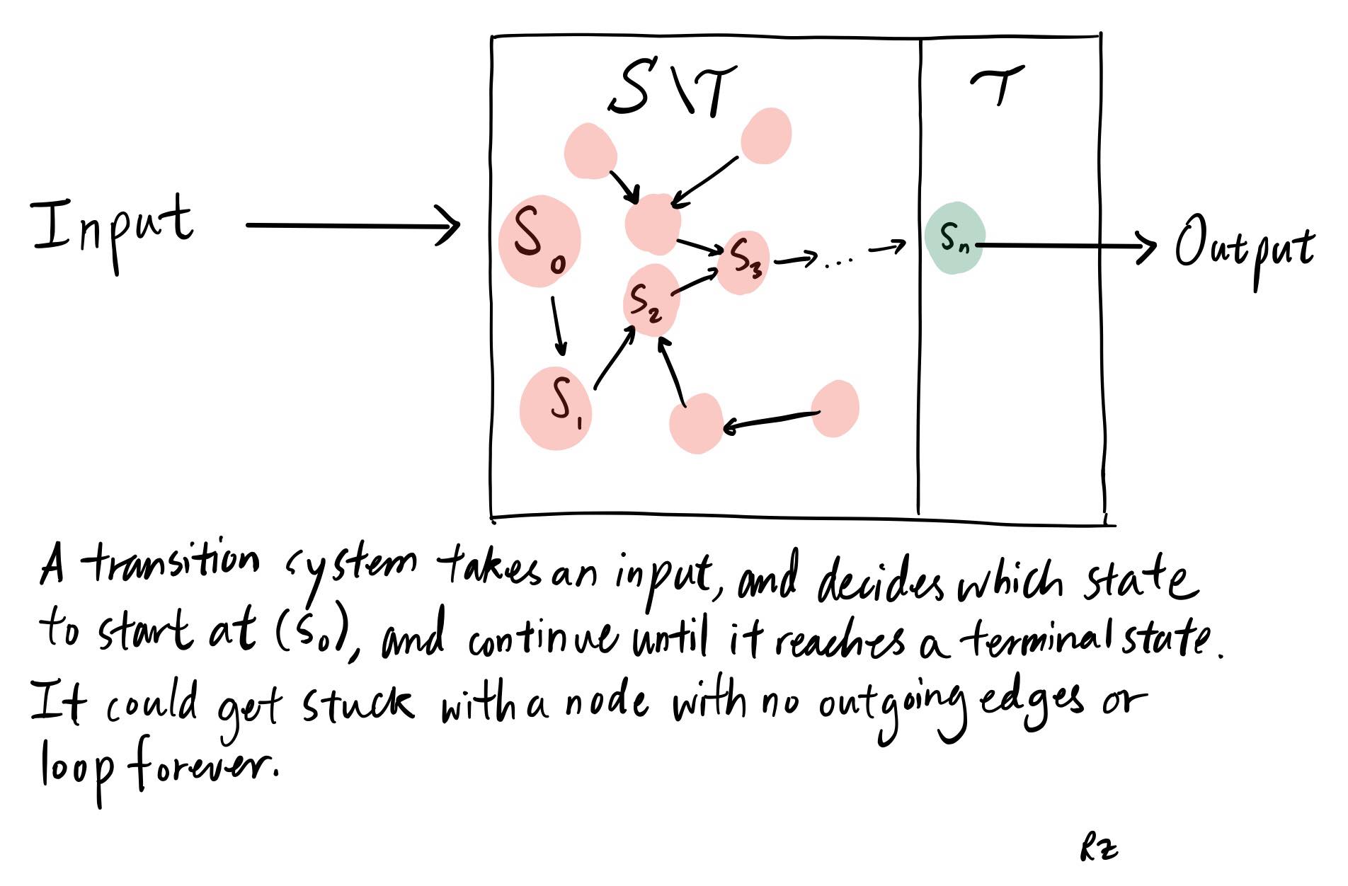
This details of this transition system can be found elsewhere, as it’s not the central point of the blog. The main take-away is that for some program
\[E \equiv \begin{cases}p_0(\vec{x}) = E_0\\p_1(\vec{x}) = E_1\\...\\p_n(\vec{x}) = E_n \end{cases}\]the program, with $\vec{x}$ substituted with actual values, can be loaded into this transition system, and the last state $t \in T$ will encode the result of the computation, which is some natural number. Sometimes, the program will run into an infinite loop, like when \(E \equiv p_0(x) = p_0(x)\) Then we won’t reach an end state - we have reached a cycle in our directed acyclic graph $\mathcal{T}$ .
In fact, just by observation, this looks like a programming language, and it is underneath the hood. Its similarities tie in more with functional languages like Haskell and OCaml more than C or Python. Then since it’s a programming language, the ability for us to parse $R(\textbf{N}_0)$ in a compiler allows us to express our compilable expressions as 0’s and 1’s. The proof that states we are able to do this is quite long and it is based off of 5-10 pages of Gödel codings, which are essentially injective mappings of some tuple $(x_1,…,x_m) = \prod_{i=1}^m p_i^{x_1+1} \in \mathbb{N}$, where $p_i$ is the $i$-th prime. This is the unique prime factorization of some number and thus the tuples’ codings must be unique. We can associate symbols with some unique tuple, which then maps to some natural number. We then create nested tuple codings to create programs injective to $\mathbb{N}$ which can be expressed in binary.
The compiler gives us some code, and our machine can take the input and return to us the result of the computation (if it doesn’t run into an infinite loop). Mathematically, we define the function $\phi(e,x)$ where $e$ is the coding for some program that calculates some partial system of equation(s). We will present the results of the code-ability of the program below.
Normal Form and Enumeration Theorem
(A part of) Kleene’s normal form states that there exists a primitive recursive function $U(y)$ and primitive recursive relation $T_n(e,x_1,…,x_n,y)$ such that a recursive partial function $f(x_1,…,x_n)$ is recursive if and only if there is some number e (the code of f) such that:
\[\exists e \in \mathbb{N}, f(\vec{x}) = U(\mu y T_n(e,\vec{x},y)) := \phi_e(x)\]One can read $T_n$ as the relation “$e$ is a program, $\vec{x}$ is the input, and $y$ is the set of states in the transition system we take until we hit a terminal state”, and one can read $U(y)$ as “$y$ is the set of states in transition system after taking in some input for some program, and $U$ retrieves the numerical value that is the output of the program”.
Recall the $\mu$ operator. This theorem states that, with two primitive recursive functions and a $\mu$ operator, we are able to create any recursive partial function from its coding, feed in the inputs, get the states of computation from the transition system, and recover the output of the function. Then, obviously, all recursive functions must be in $\mathcal{R}_\mu$. One can thus enumerate the recursive partial functions like:
\[\phi_1(x),\phi_2(x),...\]where if $e$ is not a program, $\phi_e(x) = \uparrow \forall x \in \mathbb{N}$. (It diverges because its domain is defined nowhere)
The above result shows that the set of recursive enumerable functions are countable (note at bottom*).
$S^m_n$ Theorem
The \(S^m_n\) theorem states that there exists functions \(S^m_n\) that “hardcodes” inputs into functions and returns a new function code that works as if it was hardcoded. Concretely:
- \[\forall e, y, \bar{z} = z_1,...,z_m, \bar{x} = x_1,...,x_n\]
- \[U(\mu y T_{m+n}(e,\bar{z}, \bar{x}, y)) = U(\mu yT_n(S^m_n(e,\bar{z}), \bar{x}, y))\]
- \(S^m_n\) is injective for all \(m, n\)
The proof of these theorems are difficult to explain without formal construction of the transition system and pages and pages of proofs, so just take it for face value. They’re very powerful, surprisingly. We will use the normal form’s enumerability to prove the halting problem is not recursive.
The Halting Problem
Suppose we have the halting relation $H(e,x)$ defined as:
\[X_H(e,\vec{x}) = \begin{cases}1 \quad\text{if } \phi_e(\vec{x})\downarrow \\ 0 \quad \text{else}\end{cases}\]In other words, the relation will tell us whether the program coded as $e$ in the input of $\vec{x}$ will return a result, or will diverge from endless looping or because the input was not in the domain of some partial function in the middle of the computation. Then we have the following result: The halting relation is not recursive.
Why is this true? Suppose we have an enumeration of our programs $\phi_1(\vec{x}),\phi_2(\vec{x})…$, then if $X_H(e,\vec{x})$ is recursive, then we can make a recursive function that uses it in its composition. Then let’s define one such function:
\[f(x) = \begin{cases}\phi_x(x) + 1 \quad \text{if } H(x,x) \\0 \quad \text{else}\end{cases}\]This function is obviously total, and assumed to be recursive. Here’s an illustration of what \(f\) would yield on the diagonal of this program/input matrix:
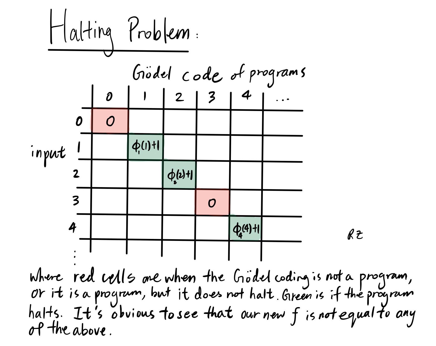
Then, $f$ can be coded up by a recursive program, which has some code $e$. What does this mean? We can feed $f$ ‘s program code, $e$, into $f$ itself, and what do we get?
\[f(e) = \phi_e(e) + 1 = f(e) + 1\]A contradiction! So then therefore $H(e,x)$ cannot be recursive, since everything else was dependent on it. This was all because we could diagonalize on all possible functions, and make this $f(x)$ different from every $g \in \mathcal{R}_\mu$. If $f$ is recursive, then $f$ would be different from itself.
Why Do You Care?
The Church-Turing thesis states that a function is computable if and only if it is recursive. That means, there does not exist an algorithm to solve specific math problems and/or philosophical problems. The expressivity of our recursive functions is very limited compared to the whole space of functions, and some age old questions are simply beyond the realm of our current model of mathematics to answer.
Note: Technically, this is an injection into $\mathbb{N}$, and to prove that it is countable we need to show that there exists an injection from $\mathbb{N}$ to $\mathcal{R}_\mu$ via Schroder-Bernstein Theorem, or to construct a bijective mapping instead into $\mathbb{N}$ instead, but since the set of recursive functions is obviously infinite, and it has to be at most countable, it’s countable.