Ray

Word embeddings are pretty amazing. But it’s not like no one knows that already.

Word embeddings are vectors that represent the latent definition of a word. They can be computed via autoencoders, or trained all the way through a classifier, like a recurrent neural net.

In this case, we trained it straight through our own implemented recurrent neural net.

The complete set of code and jupyter notebooks are in here, feel free to play around with it. Keep in mind that I implemented everything from barebone python, so it is not guaranteed to be fast for any application. I called it BibleNet because its sole purpose was to be trained on the bible corpus.

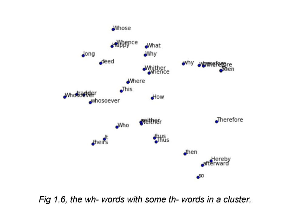
Here’s a picture of the word embeddings capturing the wh- words:

RNN Functions

These functions below are required for the RNN. Word embedding functions are what we’re using as an adhoc measure of performance, since we are evaluating how well it captures local patterns.

def sigmoid(x):
def word_embedding_forward(words, x):
def word_embedding_backward(dout, words, x):
def rnn_step_forward(prev_h, W_hh, x, W_xh, b):
def rnn_step_backward(prev_h, W_hh, x, W_xh, b, dout):
def lstm_step_forward(prev_h, W_hh, x, W_xh, b, prev_c):
def lstm_step_backward(W_hh, x, W_xh, b, cache, dh, dc):
def lstm_forward(x, W_xh, W_hh, b, h0=None):
def lstm_backward(x, W_xh, W_hh, b, h0, caches, dout):
def affine_forward(h, W_hy, b):
def affine_backward(h, W_hy, b, dout):

Optimizer

We used ADAM for optimizing the RNN, and here’s a snippet of how it works:

def adam(self, l):
    """
    adam is probably the best gradient solver in all of these selections.
    It's a combination of RMSprop and momentum.
    However, it's got a ton of configurations:
    learning_rate - standard
    beta1 - beta1 is for the momentum update
    beta2 - beta2 is for the decay rate

    m - m is the momentum
    v - v is the rmsprop cache
    """
    if self.m == None and self.v == None:
    self.v = []
    self.m = []
    [self.v.append(np.zeros_like(pair[0])) for pair in l]
    [self.m.append(np.zeros_like(pair[0])) for pair in l]
    for i, pair in enumerate(l):
        self.m[i] = self.beta1 * self.m[i] + (1.0-self.beta1)*pair[1]
        self.v[i] = self.beta2 * self.v[i] + (1.0-self.beta2)*(pair[1]**2)
        pair[0] += -1*self.learning_rate * self.m[i]/(np.sqrt(self.v[i]) + 1e-7) # 1e-7 to prevent NaN

More information on ADAM can be found in the original paper. However, it’s been shown that ADAM actually does not perform so well on the test data, compared to vanilla SGD. This may have something to do with the fact that adaptive algorithms do not do well to generalize.

Output from RNN

After training for a while, these were some example outputs:

“… matter Jazer , he indeed said , tower holy Say unto the sins of Baal , and departed not from more this , people the people of Joab king of Judah king of Judah began estimation , and told him horses , and reigned two years in Jerusalem . Wherefore the rest of the acts of Tabor , his fathers from Benhadad the word of the LORD , are they not written in the book of the chronicles of Israel ? He took the trumpet thereof . And he was the rest of the acts of Asa , and Judah to the son of Ahaziah the son of Joash displease bowls , and all the people of Israel went down , and hewed fat Damascus , and carried up the : and he took every man to the stones of Jezreel , and cakes , and had” “and Nevertheless all the gate of the beast returned unto the LORD , are they not written in the book of the chronicles of the kings of Israel in the chamber , are open : and he said , Behold , he shall not do for the LORD ; neither will we eat ? for the LORD hath done Carry him ; and borders with all the kings of Israel . The four kings at , the third year of that took incense before him , and all the sins of grant him . Chapter 9 But it came to pass , according to the prophet , and with his fathers . ******* May 4 ******* Chapter 4 Now did let us smite Israel ten years : but the LORD made him his iniquity for thee and to do for thy hand , that there was Amalekites in the field”

Not bad, but not too good. Could use some bi-lstm action or attention-based focusing using sentence embeddings or something. Note that this was a year ago and the aforementioned techniques were not ‘in the fad’.

Metric Evaluation

Both approaches were able to generate some very impressive word vectors that showed innate relationships between words. We will define the following metrics to measure how well each one did: Performance

• Exhibit meaningful general clusters
• Exhibit measurable distance between individual words for distinction of definition
• Different general clusters that are loosely connected should have similar local structures
• For each cluster, grouped by:
  • Connotation
  • Denotation
  • Part of speech

Speed

• Scalable, from 200 word vector dimensions to, say, 400.
• No large overhead

Visualization

The technique used to visualize the word embeddings will be t-SNE, which is short for t-Distributed Stochastic Neighbor Embedding, t for t-Student distribution.

It’s a famous technique used for visualization of high-dimensional data.

Because our word vectors are 4000~ dimensions large, we will definitely need to use t-SNE over a naive dimensionality reduction like the linear kernel PCA. t-SNE looks at the local details and distances of points inside of the multi-dimensional space and uses the Kullback-Leibler divergence equation to optimize this, possibly non-convex, distribution. The basic idea is that t-SNE finds the distance between $v_i$ and $v_j$ in the n-dimensional space, and minimizes the cross-entropy loss between that and the projected $v_i$ and $v_j$ in a lower, more visualizable dimension such as n = 2.

It has been shown that t-SNE performs extremely well to retain local structure.

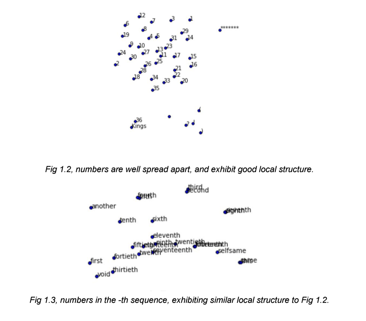
Here’s another example of how the word embedding did:

Comparison with PCA

PCA is another dimensionality reduction algorithm. It’s unsupervised, compared to our supervised word vectors, and it is a linear dimensionality reduction technique by selecting the largest eigenvalues to maximize the variance under a lower dimension.

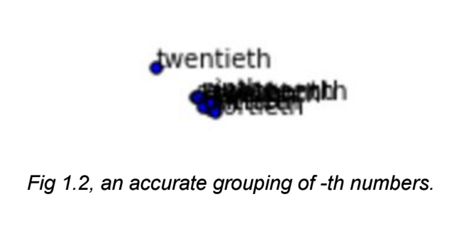
It gives us word embeddings like these(under the same t-SNE configs):

And this:

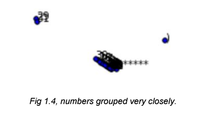
As you can see, the PCA distillation process was able to keep the relationships between the numbers close, but a little bit too close. There is no local structure, but rather PCA just assumed they were the same numbers. This dimensionality reduction technique does not explain local structure in an interpretable manner.