Previously…

Previously, we have defined the notion of a hypothesis set. We also introduced a bound that explains how far the risk of a specific hypothesis in $\mathcal{H}$ is to the optimal hypothesis $f^*$ in $\mathcal{H}$. It explains the bias variance tradeoff by illustrating that:

1. As the complexity of the model class increases, a specific hypothesis in $\mathcal{H}$ could have much worse risk than the optimal. \(|R(f)-R(f^*)|\uparrow\) \(R(f^*)\downarrow\)

2. As the complexity of the model class decreases, a specific hypothesis in $\mathcal{H}$ can’t be too far from the optimal. \(|R(f)-R(f^*)|\downarrow\) \(R(f^*)\uparrow\)

Now, let’s define the following:

\[H_m(x_1, x_2, ..., x_m) = \{(h(x_1), h(x_2), ..., h(x_m)) | h \in \mathcal{H}\}\]

$H_m(x_1, x_2, …, x_m)$ in this case is the # of possible combinations of outputs for these specific m points. If we have $\Re^{Nxd} \to \{-1,+1\}^N$, then we can have up to total $2^N$ possibilities for outputs. For example, a good $\mathcal{H}$ could give the set $\{(-1, +1), (-1, -1), (+1, -1), (+1, +1)\}$, which has a cardinality of $2^2$. We can define the following:

\[m_\mathcal{H}(N) = max_{x_{1,...,m}} |H_m(x_1,...,x_m)|\]

as the maximum cardinality of any possible combination of N outputs, of any hypothesis inside of our hypothesis set.

The maximum value for $m_\mathcal{H}(N)$ is $2^N$.

If we have $2^N$ ways to choose $N$ points, then we have all possible permutation rows, i.e.

\[\{(-1,+1)^N\}\]

Thus, initial bound:

\[m_\mathcal{H}(N) \leq 2^N \forall \mathcal{H}\]

---

VC Dimension

VC stands for Vapnik-Chervonenkis, which are the two creators of the concept. The idea of a VC dimension is that for some classifiers, there a limit to how expressive it can be.

For example, imagine a classifier on $\Re$ that predicts that everything greater than a value on the right of the line is positive, and otherwise negative. For 2 points, can we have 4 outputs? The answer is no!

Without loss of generality, assume the tuple is ordered from left to right, as in $(+1,-1)$ is negative on the left, positive on the right. This cannot be fulfilled with a classifier that says everything on the “right” is positive!

For another, cannonical example, suppose we have a linear classifier in $\Re^2$. We can have a total of 3 points classified for $2^3$ combinations, but any 4 points cannot - we cannot generate $2^4$ combinations! This is the famous XOR problem. A linear classifier cannot classifier an XOR.

An illustration of the 3 point case:

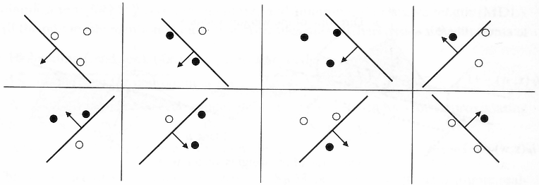
We define that for any $N$ points, $m_\mathcal{H}(N) = 2^N$, the hypothesis set shatters the dimensions.

We can then define VC as the “threshold of shatter-ability”, and we define $ VC(\mathcal{H})$ to be the maximum $N$ such that $m_\mathcal{H}(N) = 2^N$.

---

Sauer’s Lemma

Now, suppose VC dimension is $k$, then we denote a growth function $m_\mathcal{H}^k(N)$ is any growth function that cannot shatter more than k points.

\[m_\mathcal{H}^k(N) \leq \sum_i^k NCi = O(N^k)\]

which is a polynomial bound on N.

We can solve above by induction:

Denote $\mathcal{A}_{N-1}$ to be the rows that can only have a single number(1 or -1) added to the rows. It helps to think of these rows as having “saturated” its capacity given its VC dimension. If we looked at any $N$ datapoints, and saw that the hypothesis shattered them, then we must state that $VC(\mathcal{H}) \geq N$.

Denote $\mathcal{B}_{N-1}$ to be the rows that can add both a +1 and a -1.

We know that the size of our current $m_\mathcal{H}{N}$ would be defined by:

\[m_\mathcal{H}^k(N) = \mathcal{A}_{N-1} + 2\mathcal{B}_{N-1}\]

We know that since $m_\mathcal{H}^k(N)$ is built upon $m_\mathcal{H}^k(N-1)$, the rows in $m_\mathcal{H}^k(N)$ minus the last element must also be a subset of $m_\mathcal{H}^k(N-1)$:

\[m_\mathcal{H}^k(N-1) \geq \mathcal{A}_{N-1} + \mathcal{B}_{N-1}\]

We also know that $m_\mathcal{H}^{k-1}(N-1) \geq \mathcal{B}_{N-1}$, via a similar argument to our lemma. If both a $+1, -1$ can be added, then take away the $+1, -1$ and you guarantee the permutations satisfy a VC dimension of at least 1 less. This means if our permissible VC dimension was $\geq k$, it must now be $\geq k-1$.

We thus get the recurrence relation:

\[m_\mathcal{H}^k(N) \leq m_\mathcal{H}^k(N-1) + m_\mathcal{H}^{k-1}(N-1)\]

Which is elegant! We can solve this type of problem using dynamic programming, filling out a table of space $\mathcal{K} x \mathcal{N}$, or we could solve for a closed form. Luckily, we do have a closed form bound:

\[m_\mathcal{H}^k(N) \leq \sum_i^k NCi\]

This can be proven inductively. The base case is trivial, so let’s work out the inductive step:

Assume $m_\mathcal{H}^{k}(N) \leq \sum_i^{k} NCi$ and $m_\mathcal{H}^{k+1}(N) \leq \sum_i^{k+1} NCi$.

\[m_\mathcal{H}^{k+1}(N+1) \leq m_\mathcal{H}^k(N) + m_\mathcal{H}^{k+1}(N)\] \[\leq \sum_{i=0}^{k+1} NCi + \sum_{i=0}^k NCi\] \[= 1 + \sum_{i=1}^{k+1} NCi + \sum_{i=0}^k NCi\] \[= 1 + \sum_{i=0}^{k} NC(i+1) + \sum_{i=0}^k NCi\] \[= 1 + \sum_{i=0}^{k} (NC(i+1) + NCi)\] \[= 1 + \sum_{i=0}^{k} (N+1)C(i+1)\]

This step is true. You can prove it via induction or a combinatorial argument. The question is: “How many ways are there to choose $i+1$ elements from $N+1$ points?”

The answer is: “If you chose $i$ elements from $N$ points, and you chose one more on the $N+1$-th select, OR, if you chose $i+1$ elements from $N$ points, and you chose none on the $N+1$-th select.” These two events are mutually exclusive, so we will add them. We get:

\[= \sum_{i=0}^{k+1} (N+1)Ci\]

Thus we have a polynomial bound with respect to N, since $ \sum_{i=0}^{k} NCi \leq N^k$.

---

Now, we can confidently say something about our growth function $m_\mathcal{H}(N)$ - it’s $O(N^k)$. Plugging this into our original equation we get:

\[R(f) \leq [inf_{f^* \in \mathcal{H}}R(f^*)] + 2 \sqrt{\frac{log(\frac{2M}{\delta})}{2N}}\] \[= [inf_{f^* \in \mathcal{H}}R(f^*)] + 2 \sqrt{\frac{log(\frac{2m_{\mathcal{H}}(N)}{\delta})}{2N}}\] \[= [inf_{f^* \in \mathcal{H}}R(f^*)] + 2 \sqrt{\frac{log(\frac{2O(N^k)}{\delta})}{2N}}\]

And we see here that the log kills anything polynomial asymptotically, so the quantity \(\lim_{N \to \infty} \frac{log(\frac{2O(N^k)}{\delta})}{2N} \to 0\)

This is great news because then it means given a bound on the VC dimension, we can finally generalize and perform PAC learning!

---

What Just Happened?

• We learned that a common way to gauge how well a model can generalize is via Probably Approximately Correct learning. This problem formulation tells us that we are pretty accurate with a pretty good chance if we got a lot of data points.

• We expanded this idea to multiple hypotheses inside of a hypothesis set, like a set of all possible SVM’s or something similar.

• We realized that by using uniform bounds, we can say that we’re pretty accurate with a pretty good chance, for all hypotheses within our hypothesis set, as long as our hypothesis set is not that big.

  • We observed that it’s harder to be pretty accurate if our model sucks.
  • BUT, we also observed that it’s harder to have a pretty good chance if our model’s way too complicated.

• We also realized that with our uniform bound formulation, we can’t possibly extend this idea to SVM’s! There’s infinite hypotheses within the set, rendering our bound moot.

  • BUT, we also observed that if we turn our attention to a couple of points, a lot of the SVM hypotheses do effectively the same thing.
  • THEN, we realized that if our model has a special property called a VC dimension that’s finite, then we can have a better and better chance as the # of data points increase, asymptotically fulfilling PAC!

So we found out a way to prove that some models can generalize! Note that we cannot apply this idea to all models, but at least we got somewhere.

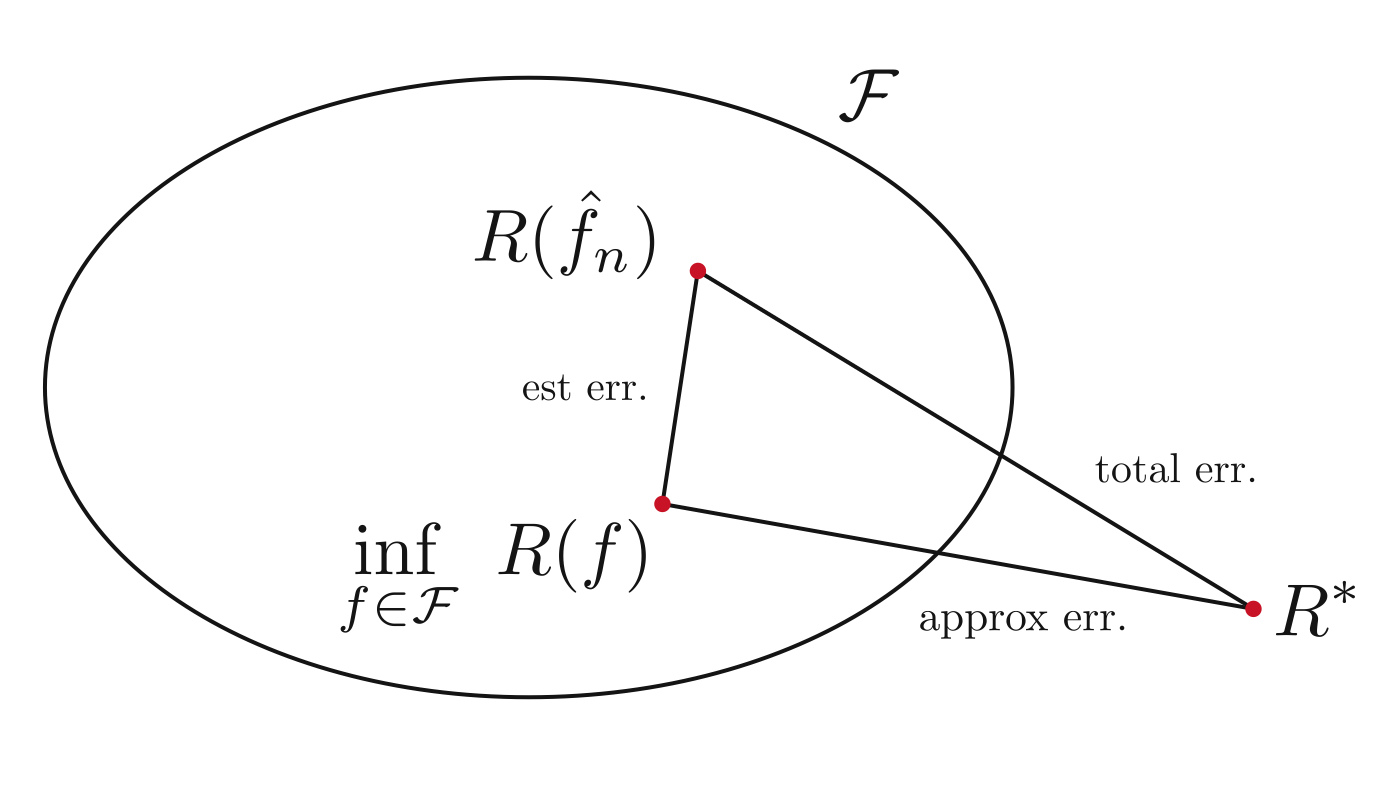
Here’s a small diagram of PAC:

---

What Else?

Rademacher Complexity

The rademacher random variable is a random variable $\sigma \in \{-1, +1\}$, with probability $\frac{1}{2}$ for each event. Consider the following:

\[E_{\sigma}[\frac{1}{N}\sum_{i=0}^N \sigma_ih(x_i)] = E_{\sigma}[h(x)] \approx E_{\sigma, D^N}[h(x)]\]

Suppose $h(x) = c \forall x$. For now we assume $h : \Re^d \to \{-1,+1\}$, then the above expression becomes:

\[\frac{1}{N}( c \sum_{i=1}^N E_{\sigma}[\sigma_i] ) = 0\]

Due to the linearity of expectation. But for a complexity class of non-shattering dimensions, we obtain $2^n$ possibilities $\forall n$. We will simply pick the hypothesis that completely overfits to the rademacher random variable noise! We can output anywhere from [-1,1], but we only care about [0,1], since negating the hypothesis that gives -1 will give us a perfect classifier. If we can arbitrarily choose $h(x_i)$ to output same sign as $\sigma_i$, then we can reach 1.

Using rademacher complexity, we can reach a similar bound as VC dimensions.

---

Thanks for sticking around! As school starts, I’ll be glancing elsewhere, hoping to learn more on the statistics side. I might come back to write one more piece on Rademacher if I have time, but I’m sure you’re all bored with learning theory already. ;)