Before we start, here’s the code:
I worked on this project with Minh Le.
Why?
You’ve probably heard this phrase “Don’t roll your own ___” thousands of times if you’re a CS major. It can be filled with crypto, standard library, parser, etc. I think nowadays, it should also contain ML library.
Regardless of this fact, it’s still an amazing lesson to learn from. People take tensorflow and similar libraries for granted nowadays; they treat it like a black box and let it run. There aren’t enough people who know what’s happening in the back. It’s really just a nonconvex optimization problem! Stop stirring the pile until it looks right.
Tensorflow
At tensorflow’s core, there is a big component that allows you to string together operations to form something called an operator graph. This operator graph is a directed graph $G = (V,E)$, where at some nodes $u_1,u_2,…,u_n,v \in V$ and $ e_1,e_2,…,e_n \in E, e_i = (u_i,v)$ we have that there exists some kind of operator that maps $ u_1,…,u_n $ to $v$.
For example, if we have x + y = z, then $(x,z), (y,z) \in E$.
This is great for evaluating the arithmetic expression. We can get the result by finding the sinks of the operator graph. Sinks are vertices such that $v \in V, \nexists e = (v, u)$. In other words, these are vertices that have no directed edges from it to anything else. Similarly, sources are $v \in V, \nexists e = (u, v)$.
For us, we will always put in values at the sources, and the values will propagate to the sinks.
Reverse-mode Differentation
Here’s some slides if you think my explanation is bad.
Differentiation is a core requirement in many of the models required in tensorflow, because we need it to run gradient descent. Everyone who graduated from highschool* knows what differentiation is; it’s just take derivatives of functions and then do chain rule if the function is a complicated composition of basic functions!
Super brief overview
If we had a function like:
\[f(x,y) = x * y\]Then differentiation with respect to x will yield:
\[\frac{df(x,y)}{dx} = y\]Then differentiation with respect to y will yield:
\[\frac{df(x,y)}{dy} = x\]Here’s another example:
\[f(x_1,x_2,...,x_n) = f(\mathbf{x}) = \mathbf{x}^T\mathbf{x}\]This derivative is just:
\[\frac{df(\mathbf{x})}{dx_i} = 2x_i\]So the gradient is just:
\[\nabla_x f(\mathbf{x}) = 2\mathbf{x}\]The chain rule, for example applied to $ f ( g ( h(x) ))$:
\[\frac{df(g(h(x)))}{dx} = \frac{df(g(h(x)))}{dg(h(x))} \frac{dg(h(x))}{dh(x)} \frac{dh(x)}{x}\]Reverse Mode in 5 Minutes
So now keep in mind the DAG structure we have for the operator graph, and the chain rule on the last example. To evaluate, we can see something like:
x -> h -> g -> f
As a graph. It will give us the answer at f. However, we can go the reversed direction as well:
dx <- dh <- dg <- df
And this will look like the chain rule! We’ll need to multiply the derivatives together on the path to get to our final result.
Here’s an example of an operator graph: 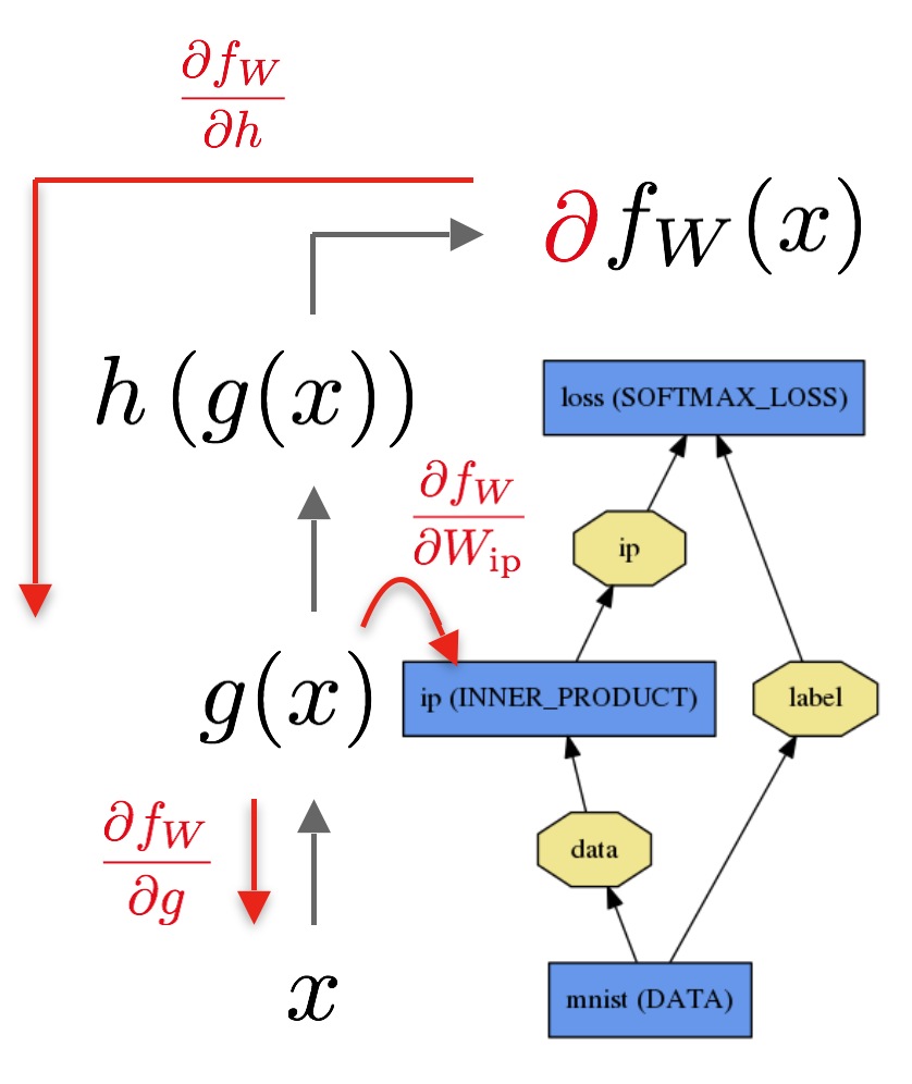
So this basically decays into a graph traversal problem. Does anyone smell topological sort and DFS/BFS?
Yup, so to support topological sort on both ways, we need to contain a set of parents and a set of children, and the sinks are sources for the other direction(vice versa).
Implementation
Before school started, Minh Le and I started designing this project. We decided to use the Eigen library backend for linear algebra operations. They have a matrix class called MatrixXd. We are using that here.
Each variable node is represented by the var class:
class var {
// Forward declaration
struct impl;

public:
    // For initialization of new vars by ptr
    var(std::shared_ptr<impl>);

    var(double);
    var(const MatrixXd&);
    var(op_type, const std::vector<var>&);
    ...

    // Access/Modify the current node value
    MatrixXd getValue() const;
    void setValue(const MatrixXd&);
    op_type getOp() const;
    void setOp(op_type);

    // Access internals (no modify)
    std::vector<var>& getChildren() const;
    std::vector<var> getParents() const;
    ...
private:
    // PImpl idiom requires forward declaration of the class:
    std::shared_ptr<impl> pimpl;
};

struct var::impl{
public:
    impl(const MatrixXd&);
    impl(op_type, const std::vector<var>&);
    MatrixXd val;
    op_type op;
    std::vector<var> children;
    std::vector<std::weak_ptr<impl>> parents;
};
In here, we employed the pImpl idiom, which means “pointer to implementation”. It’s great for many things, like decoupling implementation from interface, and allowing us to instantiate things on the heap when we have a local shell of interface on the stack. Some side-effects of pImpl are slightly slower runtime, but much shorter compile time. This allows us to keep our data structures persistent through multiple function calls/returns. A tree data structure like this should be persistent.
We have a couple enums which tells us which operations are currently being performed:
enum class op_type {
    plus,
    minus,
    multiply,
    divide,
    exponent,
    log,
    polynomial,
    dot,
    ...
    none // no operators. leaf.
};
The actual class that’s performing the evaluation of this tree is called expression:
class expression {
public:
    expression(var);
    ...
    // Recursively evaluates the tree.
    double propagate();
    ...
    // Computes the derivative for the entire graph.
    // Performs a top-down evaluation of the tree.
    void backpropagate(std::unordered_map<var, double>& leaves);
    ...
private:
    var root;
};
Inside of backpropagate, we have code that does something similar to this:
backpropagate(node, dprev):
	derivative = differentiate(node)*dprev
	for child in node.children:
		backpropagate(child, derivative)
This is pretty much doing a DFS; you see it?
Why C++?
In fact, C++ is probably not the correct language to use for this. We could’ve spent much less time developing in a functional language like OCaml. Now I realize why Scala is being used in machine learning, mainly spark ;).
However, there are obvious benefits to C++:
Eigen
For example, we can directly use tensorflow’s linear algebra library, called Eigen. It’s a template-abusing lazy-evaluation linear algebra library. Similar in flavour to our expression tree, we build up the expression, and it will only be evaluated when we really need to. However, for Eigen, they determine this during compile time,which is when templates are being used, meaning runtime is decreased. I have a lot of respect for the people who wrote Eigen, since looking at template errors make my eyes bleed.
Their code would look something like:
Matrix A(...), B(...);
auto lazy_multiply = A.dot(B);
typeid(lazy_multiply).name(); // the class name is something like Dot_Matrix_Matrix.
Matrix(lazy_multiply); // functional-style casting forces evaluation of this matrix.
The Eigen library is very powerful, and that’s why it’s one of the main backends that tensorflow uses themselves. That means there are other optimizations other than this lazy evaluation technique.
Operator Overload
Developing this library in Java would’ve been nice - no shared_ptrs, unique_ptrs, weak_ptrs; we get an actual, capable, GC. This saves development time by a lot, not to mention probably faster in execution speed as well. However, Java doesn’t allow operator overloads, and consequently they can’t have this:
// These 3 lines code up an entire neural network!
var sigm1 = 1 / (1 + exp(-1 * dot(X, w1)));
var sigm2 = 1 / (1 + exp(-1 * dot(sigm1, w2)));
var loss = sum(-1 * (y * log(sigm2) + (1-y) * log(1-sigm2)));
The above is actual code, by the way. Isn’t this extremely pretty? I would argue that this is even prettier than the python wrapper for tensorflow. And just to let you know, these are matrices, as well.
In Java, this would’ve been extremely ugly, with a bunch of add(), divide()… and et cetera. More importantly, the users would be implicitly forcing PEMDAS, which C++’s operators already exhibit very well.
Features, Not Bugs
There are some things that you can actually specify in this library that tensorflow doesn’t have clear API for, or not that I know of. For example, if we wanted to train only a specific subset of the weights, we can actually only backpropagate to the specific sources we’re interested in. This is really useful for things like transfer learning for convolutional neural nets, since many times a large net, like VGG19, is beheaded and then appended with a few extra layers of which the weights are trained according to the new domain samples.
Benchmarks
On Python’s Tensorflow library, training for 10000 epochs on the Iris dataset for classification, with the same hyperparameters, we have:
- Tensorflow’s neural net:
23812.5 ms - Scikit’s neural net library:
22412.2 ms - Autodiff’s neural net, with iterative, optimized:
25397.2 ms - Autodiff’s neural net, with iterative, no optimize:
29052.4 ms - Autodiff’s neural net, with recursive, no optimize:
28121.5 ms
So it seems, surprisingly, Scikit runs the fastest out of all of these. It may be because we’re not doing huge matrix multiplications. It may be that tensorflown had to take an extra compilation step, with variable initializers and what not. Or, it’s perhaps we had to run loops inside of python rather than in C(python loops are really bad!). I’m not sure myself.
I am fully aware that this is by no means a comprehensive benchmarking test, as it only is applied to a single data point, and in a specific situation. However, the performance of this library is not meant to be state of the art, since we don’t ever want to roll our own tensorflow.