Table of Contents

• Table of Contents
• Introduction
• Integer 8-bit quantization
  • Details
• Bitwise quantization
  • Training and Backpropagation of an XNORNet
    • Difficulty of training an XNORNet
    • Training Tips
• Approaches to Implement XNORNet
  • Forward-inference Framework
    • Linear Algebra Backend
    • Python to C++ Transpiler
  • Custom XNOR BLAS functionalities
    • xnormatmul
      • Floating point packing
      • Vectorized xnors
      • Accumulating bits
    • binConv2d

This article is WIP.

The opinions expressed in this post are my own and not necesarily those of my employer (i.e. don’t fire me pls)

Introduction

Over the summer, I interned at Airbnb’s machine learning infrastructure team, working on Airbnb’s to-be-opensourced library called Bighead. Think Uber’s Michelangelo, in that it’s an end-to-end machine learning framework, meant to wrap around most of your typical machine learning workflow, from data ingestion, to training, to hyperparameter selection, visualization, and finally deployment. When it becomes opensource, you can figure out the details for yourself.

An argument against end-to-end machine learning frameworks is that you would need to work exclusively in their environment, and for other frameworks that are not completely compliant with its API, we would need to add wrappers (like tensorflow, SpaCy, etc).

However, a similar argument for end-to-end machine learning frameworks is that because you have a homogenous wrapper interface, the user shouldn’t really care about which framework underneath they use, just that it works well, is easy to deploy, and easy to visualize and interpret.

If we have our own ecosystem, we can build our own data ingestion pipeline, optimize them however we want, and do cool things, like speed up machine learning inference by swapping out frameworks depending on which stage of the pipeline you are current executing.

The scoped context of this blog doesn’t do Bighead enough justice(there are many other features that make it a great library), so check it out when it’s available!

Integer 8-bit quantization

Nvidia has a library for forward-inference called TensorRT. It’s neat because it uses underlying GPU intrinsics for optimization (INT8 GEMM DP4A, etc), and so on Nvidia specific GPU’s, it runs very fast. Nvidia has done some work in quantizing the weights and inputs of the neural network, down from float32 to float16 or int8. For float32 to float16, you are essentially performing static_cast<float16>(float_32_number). For int8, it’s a little different:

where $Q$ and $P$ are some unknown distributions(explained later). $\gamma$ is a parameter in $P$, and we optimize the kullback-leibler convergence between these two distributions with respect to $\gamma$. The $cast_{int8}$ function is a thresholding function:

Okay, maybe it’s better expressed with code:

def cast_int8(x):
    return max(min(-127, int(x)), 127)

Now, let’s explain $Q$ and $P$.

For layers of a neural network, we usually generate these things called activation values, from functions called activation functions. The most common one is the sigmoid:

… but technically almost anything could be considered an activation function. With some data distribution $D = {x_i}_{i=0}^N$, we have some kind of activation function $f$ where $f(D) = P$. This is a generic function $f$, with some unknown distribution $D$.

Now, if we discretize all elements involved in $f$, including the input and the weights required for any operator, we get back a function $f_{int8}$, and $f_{int8}(D) * \gamma = Q_\gamma$. We minimize the KL divergence between these two distributions, $Q_\gamma$ and $P$.

TL;DR: We find the best approximation of $I^W$ with respect to $\gamma$ and the current activation function $f$.

Details

We refer to MXNet’s source code, in which I made a PR in, to explain exactly how the quantization step happens. The link to the file is here, and the PR is here.

hist, hist_edges = np.histogram(arr, bins=num_bins, range=(-th, th))
zero_bin_idx = num_bins // 2
num_half_quantized_bins = num_quantized_bins // 2
assert np.allclose(hist_edges[zero_bin_idx] + 
                   hist_edges[zero_bin_idx + 1],
                   0, rtol=1e-5, atol=1e-7)

Here, we create a histogram to approximate our activation function. The KL divergence between two continuous-valued distributions is usually performed in software via approximate binning. Each entry of the histogram is a bin entry. i.e. If you have 2 bins, then:

Because these 2 distributions are the same.

We are about to enter the important for loop that decides what threshold, i.e. $\gamma$ is optimal. We run through all reasonable $\gamma$’s and pick the one that gives the lowest KL divergence. The reasonable $\gamma$’s are between $[0, max_i(|x_i|)]$. Any elements outside of the distribution will be absorbed to the two corners of the distribution.

An example:

# Sampled numbers, sorted without loss of generality
[-10, -2, 1, 8, 12]
# If gamma = 2, and 4 bins, then we have histograms of
[|x <= -1|, |-1 < x <= 0|, |0 < x <= 1|, |1 < x|]
= [2, 0, 1, 2]

So the below is the process:

# generate reference distribution p
p = sliced_nd_hist.copy()
assert p.size % 2 == 1
assert p.size >= num_quantized_bins
# put left outlier count in p[0]
left_outlier_count = np.sum(hist[0:p_bin_idx_start])
p[0] += left_outlier_count
# put right outlier count in p[-1]
right_outlier_count = np.sum(hist[p_bin_idx_stop:])
p[-1] += right_outlier_count
# is_nonzeros[k] indicates whether hist[k] is nonzero
is_nonzeros = (p != 0).astype(np.int32)

Here, we discretize our reference distribution $P$, which is retrieved from $f(D)$. In this case, we have generated arr which is $P$. Recall that in practice, we discretize our distributions into bins so we can do a discrete KL divergence calculation.

# calculate how many bins should be merged to generate quantized distribution q
num_merged_bins = sliced_nd_hist.size // num_quantized_bins
# merge hist into num_quantized_bins bins
for j in range(num_quantized_bins):
    start = j * num_merged_bins
    stop = start + num_merged_bins
    quantized_bins[j] = sliced_nd_hist[start:stop].sum()
    
quantized_bins[-1] += sliced_nd_hist[
    num_quantized_bins * num_merged_bins:].sum()

Here, we generate our distribution $Q$, by binning up the current scope of numbers within $[-\gamma, \gamma]$ into the # of bins you can fit in an int8, which is $|[-127,-126,…,127]| = 2^8-1 = 255$ bins.

Now that we have retrieved q and p, let’s do a KL divergence on them. Using scikit:

divergence[i - num_half_quantized_bins] = stats.entropy(p, q)

And so we have found our best threshold by choosing the minimum entropy from the above expression.

There are some extra details that I left out, about smoothing the distribution to prevent divide by 0 errors and etc. Read the code for more information.

Note: The contrib folder for most frameworks is volatile, so the code above may not be an exact 1:1 at the time that you are reading it.

The performance of this model in a single GPU usually yields ~1-2x faster inference speed. On a p3.8xlarge (with 4 beefy Volta GPU’s), we can get to at most 3x faster on Resnet50. However, can we discretize this even further?

Bitwise quantization

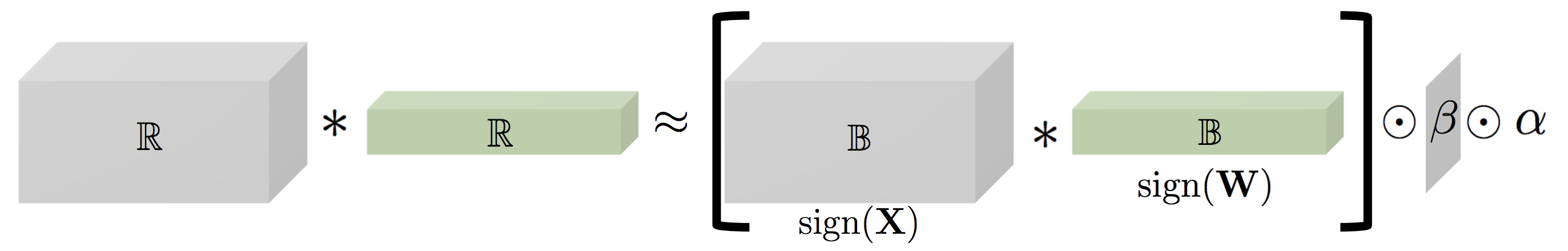
Bitwise quantization is similar to int8 quantization. The approximation is as follows:

The approximation is as follows:

One can find the best binary array and magnitudes by solving the following least squares equation:

After some calculations, the answer is (intuitively):

Multiplying two of these approximations is simple, and also leads to the optimal approximation of the two original matrices multiplied together:

And if the above were numbers:

The reason I added the number example is because matrix multiplication can be expressed as a series of dot products. If we can optimize the dot product kernel, it means we can optimize the matrix kernel as well.

If we had a number in float32:

a = [sign of a | exponent of a | mantissa of a]
a * b = [sign a XNOR sign b | exp a + exp b | mantissa a * mantissa b]

If we had a number in ${-1, +1}$, and mapped $-1$ to $0$, and $1$ to $1$ in bits:

a = [sign of a]
b = [sign of b]
a * b = a XNOR b

This means all of our multiplications can be done via XNOR’s! This means we can pack our data into bits and do a vectorized xor on multiple elements at once. This should definitely be faster than performing floating point multiplication in theory. In addition, a dot product is just a combination of multiplication and sum reduction. If we use XNOR for multiplication, we need an equivalent for sum reduction. Fortunately, there is a native intrinsic popcount instruction that allows one to count the number of 1’s in bytes(32 bytes in AVX2, 64 bytes in AVX512, etc).

A naive approach to the dot product would be:

x = ~ (a ^ b) # xnor
result = popcount(x) # popcount

which is going to be the equivalent of our dot product.

But caveat about this model is that simply doing the same conversion process as Nvidia, like discretizing to int8, will give us horrendous performance, like, random guessing performance. So our training process is going to have to be revamped.

Training and Backpropagation of an XNORNet

Where XNORNet shines is inference time. Because of the quantization of the weights and input, the forward pass of the architecture is theoretically extremely fast. However, training it is a different problem altogether.

To train an XNORNet, we actually consider the binarization function as some sort of activation function:

This means that we are actually training with floating point numbers, discretizing them in the process, and retrieving real-valued gradients for update.

This means that our backpropagation process is not going to be as fast as inference! In fact, it may be slower than normal backpropagation with floating point weights.

Difficulty of training an XNORNet

The difficult of training an XNORNet arises from the problem of discretization. Naturally, functions that discretize real values will not be continuous, and therefore it is not differentiable at every point.

Let’s look at a slightly modified sign function $sign$ or $signum$ (absorbing the case where $x$ is zero):

This function is not differentiable from the right at the point $x = 0$, and the gradient is 0 everywhere else. How can we properly backpropagate on this function?

Well, the answer is we can’t. However, Hinton(2012, Using noise as a regularizer)’s lectures introduced the idea of a straight-through estimator (STE), which is essentially arguing that the below approximation will work as a proxy for the gradient.

So therefore, if we’re performing backpropagation:

However, for practical purposes, we perform gradient clipping at this stage, and we clip with respect to the input’s magnitude, so really our gradient through the $signum$ function looks like:

Suppose we have some cost function $C$, which we are ultimately backpropagating from, then we want to know the gradient of $W$ for updates. Without loss of generality, we assume $W$ is a 1-dimensional tensor. We discretize $W \in \Re^{m}$:

Our gradient becomes:

By product rule:

Let’s tackle each piece:

And for the L-1 norm:

The final gradient should be:

Training Tips

• For input $X \approx \mathcal{B}^X * \alpha$, we can remove $\alpha$ and still yield similar accuracy. There is a roughly 3% accuracy gap.
• For the gradient, we can replace the complicated equation derived above with a simple pass-through:

and it would work just as well, but it takes longer to converge. We currently use this for inputs, but have the exact precise gradient for weights.

• As the depth of the neural network increase, the harder it is to train an XNORNet to convergence. By clipping the gradient $\forall i s.t. |X_i| \leq 1$, there may be insufficient gradient information arriving at the beginning of the neural networks. This is why several studies suggest widening the layers in an XNORNet, and why the original paper’s ResNet accuracy drops by a whopping 20% as opposed to the XNORNet version of AlexNet, which loses 10%.
• Catastrophic forgetting is a real problem in XNOR-Networks. At times the neural network will drop in training accuracy by more than 50%, and does not easily recover. Intuitively, small perturbations in the weights of the neural network drastically changes magnitude (from $-\alpha$ to $\alpha$, and vice versa), and perturbations on important parts of the weight that generate good convolution filters will cause a huge degradation in performance.
• In reality, although the optimal magnitude for approximating the matrix $W$ is expressed as follows from the least squared equation:

We have found that using $\alpha$ as a parameter for $W$ to backpropagate into also yields a similar accuracy, and reduces catastrophic forgetting (the learned $\alpha$ is usually very small).

• XNORNets are very sensitive to hyperparameters, and optimal performance requires careful handtuning or fairly exhaustive hyperparameter search, for example on the learning rate(1e-3), batch size(1024), learning rate decay(0.95), and etc. Attempts to train XNORNet without proper hyperparameters will fail to converge at all.
• One can interpret discretization as some form of regularization, and thus there is no necessary dropout layer that is further required (i.e. training accuracy usually corresponds to cross-validation accuracy).
• Clamping the weights before a forward pass between $[-1, 1]$ is a regularizer and controls gradient explosion in an XNORNet. This is also known as BinaryConnect.
• During convolution, the authors suggest averaging up each chunk of the convolution input and doing an element-wise multiplication against the final result. We found that by simply using the total average L-1 norm (a scalar), we were able to reach the same accuracy.

Although there are no proofs or bounds for why the above “hacks” yield good results and YMMV, we ended up with a test 83% accuracy on CIFAR 10 in roughly 50 epochs of 1024 batch size.

Approaches to Implement XNORNet

BLAS is a very ancient, and established linear algebra framework interface. It stands for :

• Basic
• Linear
• Algebra
• Subprograms

and many libraries implement their subroutines based off of BLAS’s interface. Some of the fastest variants of BLAS are MKL from Intel, ATLAS, and OpenBLAS. The most common subprograms deep learning uses are:

• dot (dot product between 2 vectors)
• gemv/gevm, general matrix vector
• gemm, general matrix matrix

Because many deep learning frameworks are glued to BLAS libraries, we are faced with two paths:

1. Implement a BLAS routine for bit-wise matrix multiplication, and convince some 3rd party deep learning library to incorporate our changes.
2. Make a forward-inference framework ourselves, and have the flexibility to replace gemm with xnorgemm anywhere we want.

Forward-inference Framework

Linear Algebra Backend

We wanted our library to interface directly with NumPy, which is the standard general numerical computing stack in Python along with SciPy. However, directly using NumPy will incur huge copy costs and reduced optimization, as well as the curse of GIL locking in Python.

We decided that we needed something performant and expressive, that had good bindings with NumPy, and so one of the promising candidates was xtensor, from the QuantStack team. It also had a variety of optimizations that we were looking for:

• Support for NumPy bindings
• Support for N-dimensional tensors (something that Armadillo and Eigen could not provide out-of-the-box)
• Support for lazy operators, thus reducing temporary copies and support efficient type checking using templates during compile time
• Support for black-box simd intrinsic operations
• Use modern C++11 for move semantics and compile-time generated fixed-size expressions using type traits built into the standard library.

So now we have decided on our linear algebra library and language of choice, how can we dynamically express the neural network in Python, but get it to work in C++?

Python to C++ Transpiler

As a primary goal of usability, we wanted the end-user to not spend too much time learning about our framework, but rather use their familiar Python Keras/MXNet/Tensorflow/Pytorch high-level layers, which are all similar in API. Just like how MXNet compiles its python graph into NNVM, and Tensorflow compiles its graph into LLVM, we compile our python graph into C++.

For example, we can transpile a graph in PyTorch that looks like:

ConvNet(
  (conv): Sequential(
    (0): BinaryConvolution2d()
    (1): ReLU()
    (2): MaxPool2d(kernel_size=2, stride=2, padding=0, dilation=1, ceil_mode=False)
    (3): BatchNorm2d(16, eps=1e-05, momentum=0.1, affine=True, track_running_stats=True)
    (4): BinaryConvolution2d()
    (5): ReLU()
    (6): MaxPool2d(kernel_size=2, stride=2, padding=0, dilation=1, ceil_mode=False)
    (7): BatchNorm2d(32, eps=1e-05, momentum=0.1, affine=True, track_running_stats=True)
  )
  (fc): BinaryLinear()
)

into some C++ code that looks like:

...

extern "C" {
auto&& Block__0BinaryConv2d__weight = getParameter<float>("Block__0BinaryConv2d__weight");
auto&& Block__0BinaryConv2d__bias = getParameter<float>("Block__0BinaryConv2d__bias");
auto&& Block__3BatchNorm__gamma = getParameter<float>("Block__3BatchNorm__gamma");
auto&& Block__3BatchNorm__beta = getParameter<float>("Block__3BatchNorm__beta");
auto&& Block__3BatchNorm__running_mean = getParameter<float>("Block__3BatchNorm__running_mean");
auto&& Block__3BatchNorm__running_var = getParameter<float>("Block__3BatchNorm__running_var");
static constexpr float Block__3BatchNorm__epsilon = 1e-05;
auto&& Block__4BinaryConv2d__weight = getParameter<float>("Block__4BinaryConv2d__weight");
auto&& Block__4BinaryConv2d__bias = getParameter<float>("Block__4BinaryConv2d__bias");
auto&& Block__7BatchNorm__gamma = getParameter<float>("Block__7BatchNorm__gamma");
auto&& Block__7BatchNorm__beta = getParameter<float>("Block__7BatchNorm__beta");
auto&& Block__7BatchNorm__running_mean = getParameter<float>("Block__7BatchNorm__running_mean");
auto&& Block__7BatchNorm__running_var = getParameter<float>("Block__7BatchNorm__running_var");
static constexpr float Block__7BatchNorm__epsilon = 1e-05;
auto&& Block__9BinaryDense__weight = getParameter<float>("Block__9BinaryDense__weight");
auto&& Block__9BinaryDense__bias = getParameter<float>("Block__9BinaryDense__bias");

xt::xarray<float> transform(const xt::xarray<float>& batch, const std::string& prefix){
	xt::xarray<float> result;
	auto in_shape = batch.shape()[0];
	auto rows = std::min(in_shape, decltype(in_shape)(60000));
	result.resize({ rows, 10 });
	#pragma omp parallel for
	for(auto i = 0; i < rows; i++){
		auto&& data = xt::view(batch, xt::range(i, i+1));
		auto&& Block__0BinaryConv2d__binConv2d = bighead::linalg::conv::binConv2d(data, Block__0BinaryConv2d__weight, 1, 0);
		auto&& Block__0BinaryConv2d__binConv2d_bias = Block__0BinaryConv2d__binConv2d + xt::view(Block__0BinaryConv2d__bias, xt::newaxis(), xt::all(), xt::newaxis(), xt::newaxis());
		auto&& Block__1ReLU__relu = Block__0BinaryConv2d__binConv2d_bias * xt::cast<float>(0 < Block__0BinaryConv2d__binConv2d_bias);
		auto&& Block__2MaxPool2d__maxPool2d = bighead::linalg::pool::maxPool2d(Block__1ReLU__relu, 2, 2, 0);
		auto&& Block__3BatchNorm__batchNormgamma = xt::view(Block__3BatchNorm__gamma, xt::newaxis(), xt::all(), xt::newaxis(), xt::newaxis());
		auto&& Block__3BatchNorm__batchNormbeta = xt::view(Block__3BatchNorm__beta, xt::newaxis(), xt::all(), xt::newaxis(), xt::newaxis());
		auto&& Block__3BatchNorm__batchNormrunning_mean = xt::view(Block__3BatchNorm__running_mean, xt::newaxis(), xt::all(), xt::newaxis(), xt::newaxis());
		auto&& Block__3BatchNorm__batchNormrunning_var = xt::view(Block__3BatchNorm__running_var, xt::newaxis(), xt::all(), xt::newaxis(), xt::newaxis());
		auto&& Block__3BatchNorm__batchNorm = Block__3BatchNorm__batchNormgamma * (Block__2MaxPool2d__maxPool2d - Block__3BatchNorm__batchNormrunning_mean) / xt::sqrt(Block__3BatchNorm__batchNormrunning_var + Block__3BatchNorm__epsilon) + Block__3BatchNorm__batchNormbeta;
		auto&& Block__4BinaryConv2d__binConv2d = bighead::linalg::conv::binConv2d(Block__3BatchNorm__batchNorm, Block__4BinaryConv2d__weight, 1, 0);
		auto&& Block__4BinaryConv2d__binConv2d_bias = Block__4BinaryConv2d__binConv2d + xt::view(Block__4BinaryConv2d__bias, xt::newaxis(), xt::all(), xt::newaxis(), xt::newaxis());
		auto&& Block__5ReLU__relu = Block__4BinaryConv2d__binConv2d_bias * xt::cast<float>(0 < Block__4BinaryConv2d__binConv2d_bias);
		auto&& Block__6MaxPool2d__maxPool2d = bighead::linalg::pool::maxPool2d(Block__5ReLU__relu, 2, 2, 0);
		auto&& Block__7BatchNorm__batchNormgamma = xt::view(Block__7BatchNorm__gamma, xt::newaxis(), xt::all(), xt::newaxis(), xt::newaxis());
		auto&& Block__7BatchNorm__batchNormbeta = xt::view(Block__7BatchNorm__beta, xt::newaxis(), xt::all(), xt::newaxis(), xt::newaxis());
		auto&& Block__7BatchNorm__batchNormrunning_mean = xt::view(Block__7BatchNorm__running_mean, xt::newaxis(), xt::all(), xt::newaxis(), xt::newaxis());
		auto&& Block__7BatchNorm__batchNormrunning_var = xt::view(Block__7BatchNorm__running_var, xt::newaxis(), xt::all(), xt::newaxis(), xt::newaxis());
		auto&& Block__7BatchNorm__batchNorm = Block__7BatchNorm__batchNormgamma * (Block__6MaxPool2d__maxPool2d - Block__7BatchNorm__batchNormrunning_mean) / xt::sqrt(Block__7BatchNorm__batchNormrunning_var + Block__7BatchNorm__epsilon) + Block__7BatchNorm__batchNormbeta;
		auto&& Block__8Flatten__reshape = xt::eval(Block__7BatchNorm__batchNorm);
		Block__8Flatten__reshape.reshape({ Block__8Flatten__reshape.shape()[0], 512 });
		auto&& Block__9BinaryDense__xnorAffine = bighead::linalg::xnor::xnormatmul(Block__8Flatten__reshape, Block__9BinaryDense__weight);
		auto&& Block__9BinaryDense__xnorAffine_bias = Block__9BinaryDense__xnorAffine + xt::view(Block__9BinaryDense__bias, xt::newaxis(), xt::all());
		xt::view(result, xt::range(i,i+1)) = std::forward<decltype(Block__9BinaryDense__xnorAffine_bias)>(Block__9BinaryDense__xnorAffine_bias);
	}
	return result;
}
...
} // extern "C"

One advantage that a C++ transpiler has over something like tensorflow’s LLVM compiler is that we can easily inspect the C++ code for bugs during a model-building iteration cycle.

Because C++ is an easier barrier to entry, others could easily implement layers that would compile C++ code as long as they knew how to use the linear algebra backend(for e.x. xtensor). The fact that the layers could technically emit anything means that fellow python/C++ programmers can expand the backend emitter usage to more than just deep learning applications, but rather other parts of the data processing pipeline. In the future, we hope to compile all parts of the bighead pipeline into C++ wherever possible, so we can offer blazing fast performance after a single fit() call.

Custom XNOR BLAS functionalities

xnormatmul

bighead::linalg::xnor::xnormatmul is our level 3 BLAS routine that takes in any lazily evaluated xt::xexpression<T> matrix A and xt::xexpression<O> matrix B. The multiplication between the two is done via special compiler intrinsics. For our purposes, we implemented it with vectorized instructions in mind, specifically AVX2. It consists of 3 stages:

1. quantization stage - taking floating point numbers inside of a matrix and compressing it into signed bits (0 for -1, 1 for 1).
2. multiplication stage - instead of performing floating point multiplications, we use vectorized XNOR on all elements.
3. accumulation stage - perform a popcount (pop stands for population) on the resulting xnor’d vector and write it into the resulting matrix.

Floating point packing

A floating point number consists of 3 parts: sign bit, exponent, fraction. The sign bit is a 0 if the number is negative, and 1 if the number is positive. If we can extract this part of every floating point number, then our life would be very easy.

Luckily, we even have a vectorized instruction (in AVX2) for this:

_mm256_movemask_ps, which roughly gets compiled to vpmovmskb <reg> <ymm reg> where reg means register.

The above instruction takes the first bit of the next eight single precision floating points and packs them into a single byte. This is exactly what we need in order to pack the data.

We also make sure that the container of which we use to pack the data is aligned. We use the xsimd::aligned_allocator<std::uint8_t, 32> to align the pointer of our array so that the condition std::reinterpret_cast<intptr_t>(ptr) % 32 is always true for any bitmap we use. We need aligned instructions so that we can have safe loading for our consequent instructions below. (Note that aligned vs. unaligned instructions for loading may have very marginal difference depending on the architecture, but we decided to force alignment regardless)

Vectorized xnors

Given the bit-packed data, we can perform a bit-flip operation(~a) on the xor result(a^b). We can use _mm256_load_si256 and _mm256_store_si256 to perform these operators on 256 bits of data at once.

Accumulating bits

After xnor’ing the two operands, we can scan through the resulting matrix and return the total number of 1’s we see. There is a routine called popcount that performs exactly what we want. However, this only exists in AVX512, specifically the _mm512_popcnt_epi32 and its corresponding variants. In this case, we implement the Hamming weight (or Harley-Seal) algorithm which performs the following to compute number of bits in AVX2:

...
// For purposes of illustration, we express ints as binary
int x = 00100110; // result should be 3
temp0 = x & 01010101; // 00000100
temp1 = (x >> 1) & 01010101; // 00010001 
res = temp0 + temp1; // 00010101
temp0 = res & 00110011; // 00010001
temp1 = (res >> 2) & 00110011; // 00000001
res = temp0 + temp1; // 00010010
temp0 = res & 00001111; // 00000010
temp1 = (res >> 4) & 00001111; // 00000001
res = temp0 + temp1; // 00000011 = 3 bits.

The rationale behind the algorithm is that it is computing, at every iteration, a container that holds 4 2-bit numbers, 2 4-bit numbers, and 1 8-bit number, each of which contains number of bits which added up together into the 8-bit number is the popcount. We use a total of 12 operations, all of which are inexpensive. We have vectorized instructions for addition, AND, and shifting, so we are effectively using 12 operations on 256 bits at once.

binConv2d

For example, in the above transpilation, we transpiled the BinaryConvolution2d into bighead::linalg::conv::binConv2d in C++. For all functions within the namespace bighead, they are functions implemented by the Bighead team. binConv2d is a function that performs convolutions with binary weights and inputs, like so:

In the XNORNet paper, the authors suggested to take the average magnitude of each convolution input and multiply the resulting filters element-wise against the magnitudes. However, the authors of DoReFa networks and ReBNetworks show that a single scalar of the average magnitude of the entire input, multiplied via broadcasting will work just as well. We adopt the latter approach in our implementation.