Table of Contents
- Table of Contents
- Temporal Difference Prediction
- Optimality of TD(0)
- On-policy: Sarsa
- Off-policy: Q-learning
- Example: Cliff Walking
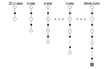
Temporal difference learning is one of the most central concepts to reinforcement learning. It is a combination of Monte Carlo ideas [todo link], and dynamic programming [todo link] as we had previously discussed.
Review of Monte Carlo
In Monte Carlo, we have an update rule to capture the expected rewards $V$ under a given policy $\pi$. Usually, we simulate entire episodes and get the total reward, and attribute each action in the action sequence to the reward value. Recall we had two different ways of Monte Carlo simulation - every-visit and first-visit.
Given some state sequence $S_j = (s_0, s_1, …)$, and action sequence $A_j = (a_0, a_1, …)$ belonging to some episode $j$, first-visit MC will perform the following:
\[V(s) = \frac{1}{N}\sum_{i:s \in S_i}^N G^i_{min_j\{s_j | s_j = s\}}\]For some reward $G^i_t$ which is the (possibly discounted) sum of subsequent rewards in episode $i$ after time $t$. In other words, if a state occurs once, or twice, or fifty times throughout an episode, we only count the first occurence of the state. and average all of the reward values for $V_s$. For every-visit MC, we have:
\[\mathcal{G}^i_s = \sum_{j:s_j = s, s_j \in S_i \forall S_i} G^i_j \\ V(s) = \frac{1}{\#s} \sum_i^M \mathcal{G}^i_s\]where #s is the total number of times we saw state $s$ throughout all episodes. In other words, if a state occurs more than once, we will add those occurences into our value approximation and average all the rewards values to get $V(s)$.
In many cases, $V(s)$ is stationary, and both methods (first-visit and every-visit) will converge to the optimal answer. However, in a nonstationary environment, we do not want our “update magnitude” to approach 0. The below is an update rule suitable for a nonstationary, every-visit MC (eq. 0):
\[V(S_t) = V(S_t) + \alpha [ G_t - V(S_t) ]\]for some constant $\alpha > 0$.
Temporal Difference Prediction
In the above equation, we use the quantity $G_t$, which is the rewards for the rest of the episode following time $t$, possibly discounted by some factor $\gamma$. This quantity is only known once the episode ends. For TD, this is no longer necessary!
How does TD methods do this? They only need to look at one step ahead, because their approximation is slightly less precise and less sample-based. Instead of $G_t$, they use:
\[R_{t+1} + \gamma V(S_{t+1})\]Recall that the equation for $G_t$ is:
\[G_t = \sum_{k=t+1} \gamma^{k-t-1}R_k = R_{t+1} + \gamma R_{t+2} + \gamma^2 R_{t+3} + ...\]And the equation for $V(S_t)$ is:
\[V(S_t) = E[G_t]\]And so we’re sort of “approximating” the rest of the trajectories:
\[V(S_{t+1}) = E[R_{t+2} + \gamma R_{t+3} + ...] \approx R_{t+2} + \gamma R_{t+3} + ...\]So yes, it is less precise, but in return, we are able to learn in the middle of an episode. The resulting update equation for $V(S_t)$ in the analog of $\text{eq (0)}$ is:
\[V(S_t) = V(S_t) + \alpha [ R_{t+1} + \gamma V(S_{t+1}) - V(S_t) ]\]In this case, since we’re only looking one step ahead, it is called $TD(0)$. Here’s some pseudocode logic:
pi = init_pi()
V = init_V()
for i in range(NUM_ITER):
    s = init_state()
    episode = init_episode(s)
    while episode:
        prev_s = s
        action = get_action(pi, V)
        reward, s = episode.run(action)
        V(prev_s) += alpha * (reward + gamma * V(s) - V(prev_s))
$TD(0)$ is considered a bootstrapping method because it uses previous approximations, rather than completely using the entire trajectory’s reward.
Similarity between TD and DP
Recall that dynamic programming approaches to solve reinforcement learning problems uses the Bellman backup operator. This allows efficient incremental computation of $V(s)$, and we previously proved that $lim_{k \to \infty} v_k(s) = v_\pi(s)$. In this way, we are effectively getting more and more accurate approximations of $v$.
In a similar nature, our approximation of $V(S_t)$ in the equation above is also iterative, and bootstraps off of the previous estimation, because $V(S_t)$ as a function is not known.
Similarity between TD and Monte Carlo
Recall that Monte Carlo requires us to estimate the expected value, because we’re taking samples of episodes and trying to approximate the underlying expected value from each action. In this way, TD acts like a every-visit MC due to its $V(S_t)$ being an approximation to the expected value of $G_t$.
Thus, TD and Monte Carlo both approximate $V(S_t)$ via sampling because the expectation is not known. However, Monte Carlo does not attempt to use previous estimations of $V$ in its convergence; instead, it takes the complete sample trajectory to estimate.
Optimality of TD(0)
One might expect TD(0) to converge to the same value as monte carlo methods. However, this is not true. Sutton’s pathological example explains this very clearly:
| Trials | Rewards |
|---|---|
| A, B | 0, 0 |
| B | 0 |
| B | 1 |
| B | 1 |
| B | 1 |
| B | 1 |
| B | 1 |
| B | 1 |
For these episodes, we have 6 episodes where B resulted in a reward of 1, and 2 episodes where it resulted in 0. Therefore, we can safely say that $V(B) = \frac{3}{4}$.
We can make 2 “reasonable” suggestions about A:
- When
Aoccurred, the resulting accumulated reward $G$ is 0. Therefore, $V(A) = 0$. - When
Aoccurred, the resulting next state is alwaysB. Therefore, since $V(A) = E(R_{t+1} + \gamma R_{t+2} + … ) \approx 0 + \gamma V(B)$, since the only next state is $B$, and our current reward is 0 from the single sample we have, the result should be $0 + \gamma V(B) = \frac{3 \gamma}{4} \neq 0$. This makes sense from the Markovian assumption, since $S_t \perp R_{t+2}$, so the fact that $A$ happened before $B$ should not cause $B$ to yield a reward of $0$.
In a sense, Monte Carlo minimizes the value function approximation’s mean squared error, meanwhile TD converges towards the certainty-equivalence estimate. The certainty-equivalence estimate is the maximum likelihood estimate of the value function under the assumption that the process is MDP.
On-policy: Sarsa
In an on-policy setting, we learn an action-value function $q(s,a)$ rather than $v(s)$ discussed above. The generalization is quite straightforward:
\[Q(S_t, A_t) = Q(S_t, A_t) + \alpha [ R_{t+1} + \gamma Q(S_{t+1}, A_{t+1}) - Q(S_t, A_t)]\]As opposed to:
\[V(S_t) = V(S_t) + \alpha [ R_{t+1} + \gamma V(S_{t+1}) - V(S_t)]\]The reason we call this algorithm Sarsa is because it is a sequence of State, Action, Reward, State, Action. Just like any on-policy RL algorithm, we estimate $q_\pi$ for some $\pi$. This $\pi$ is some policy that outputs probability of actions based off of the current state.
As always, on-policy algorithms may not explore enough of the search space and lead to a suboptimal answer, or get stuck in its current policy forever and fail to terminate. As a result, we usually use $\epsilon$-greedy policy $\pi$, to select all other actions with a small probability $\epsilon$.
Off-policy: Q-learning
The corresponding off-policy variant of Sarsa is called Q-learning, and it is defined by the update rule:
\[Q(S_t, A_t) = Q(S_t, A_t) + \alpha [ R_{t+1} + \gamma max_a Q(S_{t+1}, a) - Q(S_t, A_t) ]\]The only difference here is that instead of approximating $G_t$ with $R_{t+1} + \gamma Q(S_{t+1}, A_{t+1})$, in which $A_{t+1}$ is picked from an $\epsilon$-greedy policy, we are picking the actual optimal action which is $max_a Q(S_{t+1}, a)$. This is an off-policy TD control algorithm because we are using $\epsilon$-greedy for simulation, but we are approximating $Q$ with the actual $argmax$.
Example: Cliff Walking
Once again, let’s take the previous Cliff Walking gym we used for Monte Carlo methods. As we had previously observed, the converged path on the graph was:
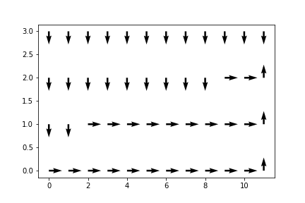
This was for an on-policy Monte Carlo method. The reason for the path being so conservative, and the actor moving all the way up to the edge was due to the fact that there was $\epsilon$ probability that the actor would’ve moved in a random direction, one which will kill the actor. Even as $\epsilon$ approached 0, the strategy is not optimal, but extremely safe.
Now, I have added the TD functionality in the same Monte Carlo repository (now named RLModels), and refactored most of the core functionality. We directly translate the update rules above into the update_Q() function, and we pass in the tuple (state, action, reward, state, action) instead of an episode, i.e. [(state, action, reward), ...]:
Sarsa Model
For Sarsa, we use the update rule:
\[Q(S_t, A_t) = Q(S_t, A_t) + \alpha [ R_{t+1} + \gamma Q(S_{t+1}, A_{t+1}) - Q(S_t, A_t)]\]per event in an episode. We reflect that in our model below.
class FiniteSarsaModel(FiniteModel):
    def __init__(self, state_space, action_space, gamma=1.0, epsilon=0.1, alpha=0.01):
        """SarsaModel takes in state_space and action_space (finite)
        Arguments
        ---------

        state_space: int OR list[observation], where observation is any hashable type from env's obs.
        action_space: int OR list[action], where action is any hashable type from env's actions.
        gamma: float, discounting factor.
        epsilon: float, epsilon-greedy parameter.

        If the parameter is an int, then we generate a list, and otherwise we generate a dictionary.
        >>> m = FiniteSarsaModel(2,3,epsilon=0)
        >>> m.Q
        [[0, 0, 0], [0, 0, 0]]
        >>> m.Q[0][1] = 1
        >>> m.Q
        [[0, 1, 0], [0, 0, 0]]
        >>> m.pi(1, 0)
        1
        >>> m.pi(1, 1)
        0
        """
        super(FiniteSarsaModel, self).__init__(state_space, action_space, gamma, epsilon)
        self.alpha = alpha


    def update_Q(self, sarsa):
        """Performs a TD(0) action-value update using a single step.
        Arguments
        ---------

        sarsa: (state, action, reward, state, action), an event in an episode.
        """
        # Generate returns, return ratio
        p_state, p_action, reward, n_state, n_action = sarsa
        q = self.Q[p_state][p_action]
        self.Q[p_state][p_action] = q + self.alpha * \
            (reward + self.gamma * self.Q[n_state][n_action] - q)


    def score(self, env, policy, n_samples=1000):
        """Evaluates a specific policy with regards to the env.
        Arguments
        ---------

        env: an openai gym env, or anything that follows the api.
        policy: a function, could be self.pi, self.b, etc.
        """
        rewards = []
        for _ in range(n_samples):
            observation = env.reset()
            cum_rewards = 0
            while True:
                action = self.choose_action(policy, observation)
                observation, reward, done, _ = env.step(action)
                cum_rewards += reward
                if done:
                    rewards.append(cum_rewards)
                    break
        return np.mean(rewards)
Q-Learning Model
For Q-learning, we use an argmax variant of Sarsa, to make it an off-policy model. The update rule looks like:
\[Q(S_t, A_t) = Q(S_t, A_t) + \alpha [ R_{t+1} + \gamma max_a Q(S_{t+1}, a) - Q(S_t, A_t) ]\]Here is the model in python:
class FiniteQLearningModel(FiniteModel):
    def __init__(self, state_space, action_space, gamma=1.0, epsilon=0.1, alpha=0.01):
        """FiniteQLearningModel takes in state_space and action_space (finite)
        Arguments
        ---------

        state_space: int OR list[observation], where observation is any hashable type from env's obs.
        action_space: int OR list[action], where action is any hashable type from env's actions.
        gamma: float, discounting factor.
        epsilon: float, epsilon-greedy parameter.

        If the parameter is an int, then we generate a list, and otherwise we generate a dictionary.
        >>> m = FiniteQLearningModel(2,3,epsilon=0)
        >>> m.Q
        [[0, 0, 0], [0, 0, 0]]
        >>> m.Q[0][1] = 1
        >>> m.Q
        [[0, 1, 0], [0, 0, 0]]
        >>> m.pi(1, 0)
        1
        >>> m.pi(1, 1)
        0
        """
        super(FiniteQLearningModel, self).__init__(state_space, action_space, gamma, epsilon)
        self.alpha = alpha


    def update_Q(self, sars):
        """Performs a TD(0) action-value update using a single step.
        Arguments
        ---------

        sars: (state, action, reward, state, action) or (state, action, reward, state),
            an event in an episode.

        NOTE: For Q-Learning, we don't actually use the next action, since we argmax.
        """
        # Generate returns, return ratio
        if len(sars) > 4:
            sars = sars[:4]

        p_state, p_action, reward, n_state = sars
        q = self.Q[p_state][p_action]
        max_q = max(self.Q[n_state].values()) if isinstance(self.Q[n_state], dict) else max(self.Q[n_state])
        self.Q[p_state][p_action] = q + self.alpha * \
            (reward + self.gamma * max_q - q)


    def score(self, env, policy, n_samples=1000):
        """Evaluates a specific policy with regards to the env.
        Arguments
        ---------

        env: an openai gym env, or anything that follows the api.
        policy: a function, could be self.pi, self.b, etc.
        """
        rewards = []
        for _ in range(n_samples):
            observation = env.reset()
            cum_rewards = 0
            while True:
                action = self.choose_action(policy, observation)
                observation, reward, done, _ = env.step(action)
                cum_rewards += reward
                if done:
                    rewards.append(cum_rewards)
                    break
        return np.mean(rewards)


if __name__ == "__main__":
    import doctest
    doctest.testmod()
Cliffwalking Maps
By running the two models above, we get different cliffwalking maps:
For SARSA:
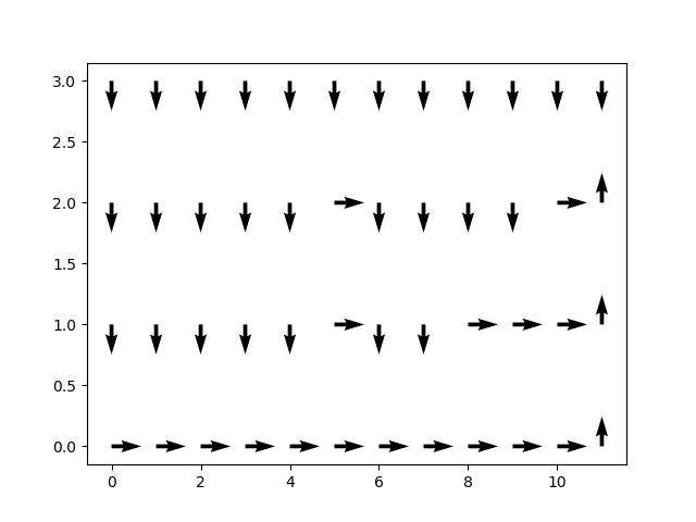
As we can see, it is similar to that of Monte Carlo’s map. The action is conservative because it does not assume any markovian structure of the process. The Monte Carlo process is actively aware of the stochasticity in the environment and tries to move to the safest corner before proceeding to the right and ultimately to the end.
For Q-learning:
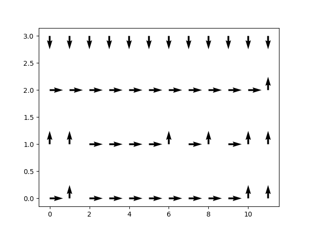
This is a very different map compared to SARSA and Monte Carlo. Q-Learning understands the underlying markovian assumption and thus ignores the stochasticity in choosing its actions, hence why it picks the optimal route (the reason it understands the markovian assumption is that it picks the greedy action, which is optimal under the Strong Markov Property of the MDP). The off-policy approach allows Q-Learning to have a policy that is optimal while its $\epsilon$-greedy simulations allows it to explore.
In my opinion, Q-learning wins this round.
Learning Curves
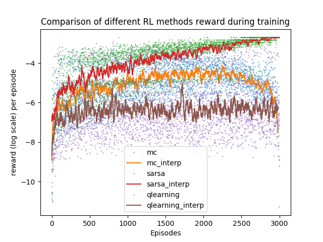
We run all three models in tandem, and we record the total reward per episode for each of the techniques as epochs increase. The *_interp are moving averages of the log rewards. It appears that SARSA, although producing approximately the same solution as Monte Carlo (recall that it is not exact), converges to a higher reward much faster. This is due to the fact that its value function was able to be updated per step rather than per episode. This method of bootstrapping allows the model to learn a lot faster than Monte Carlo.
Another observation we can see is that Q-learning’s average reward is bad. This is due to the fact that Q-learning tries to take the optimal action, but gets screwed over by the $\epsilon$ probability of falling off a cliff due to the stochasticity of the $\epsilon$-greedy policy that it uses to explore.
Another interesting phenomenon observed in the above diagram is that Monte Carlo actually starts to degrade in performance near the end. This… I have no explanation for (and I’d love to discuss it!).