Preface
If you haven’t seen the previous blog, or not familiar with Hoeffding bounds, I suggest you read about it. This blog goes head first into the continuation of the previous blog here.
What is a hypothesis?
A hypothesis, can be thought of as a function. However, it’s not necessary. A function maps something to something else, like $f: \Re^n \to \Re$. For every input in the domain, we know there exists a single output. However, in our world of unknowns, it’s not known whether a point will map to more than one coordinate, depending on the underlying noise.
Our definition of noise, is the unknown consequences of the outside environment that we failed to capture in our data mining. This noise makes the deterministic idea of a function fall apart, so instead of:
\[f(x_n)\]We now take the stochastic analog:
\[p(y_n|x_n)\]Which gives us a probability distribution of all outputs. Instead of a mapping of $f: \Re^n \to \Re$, for example, it is now $X: \Omega \to \Re$, where $\Omega$ is the set of all events.
A hypothesis in our case is just a mathematical model that tries to map x’s to y’s with a probability associated with it, or a transformation of a random variable. Hypotheses are motivated with reasonable assumptions:
- linear regression assumes a linear mapping $f$ between x and y with gaussian noise.
- linear support vector machine assumes a separating hyperplane with greatest margin between two classes.
- logistic regression assumes a separating hyperplane with the sigmoid function modeling the bernoulli distribution.
- decision trees assume that the data is separated into classes by parallel axis splits, of which minimize the entropy/misclassification/gini index/etc.
- neural networks assume a nonlinear mapping between x and y, and attempts to model the probability distribution underneath. In reality, neural networks are just self-learned kernel functions of the data applied to a linear model. There’s nothing special.
And the list goes on.
But be careful, you can’t say “linear models” is a hypothesis. It’s too broad - we need to specify the specific weights, i.e. “linear model with coefficients $x0 = 1$, $x1 = 0.2$, etc.”. Thus, we call “linear models” a hypothesis set, containing many hypotheses.
Recap
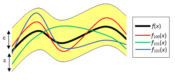
Hoeffding, as we talked about before, tries to analyze the bound of the difference between the empirical risk and the expected risk of a hypothesis, $f$.
What we managed to get was:
\[P(|R_{N}(f) - R(f)| > \epsilon) \leq 2e^{-2N\epsilon^2}\]This gives us confidence about whether our model, trained on our training data, will be able to generalize, and express the underlying data distribution, $x, y \sim p_\theta$.
This is great and all, but this is only one hypothesis. For a general class of hypotheses, like support vectors, how can we make a similar argument?
Uniform Bound
The most basic way to plug Hoeffding into a general class of hypothesis, which we will denote $ \mathcal{H} $, is to assume that there exists no overlap between the bad hypotheses(I will elaborate on what overlap means). A bad hypothesis is one where:
\[|R_{N}(f_{bad}) - R(f_{bad})| \geq \epsilon\]for some $\epsilon$.
This event can happen to any of the hypotheses in our set of hypotheses. So if our hypothesis set has cardinality $|\mathcal{H}| = M$ , then we have $M$ of these events that we have to avoid. If we define the event of i-th hypothesis being bad as
\[B_i = \{|R_{N}(f_i) - R(f_i)| \geq \epsilon\}\]Then the event that none of the hypotheses are bad is: $ {\bigcap_{i=0}^M B_i^c} $ , which translates to
“The 1st hypothesis is NOT bad AND the 2nd hypothesis is NOT bad AND…”
If we apply De Morgan’s law to this, we get:
\[\{\bigcap_{i=0}^M (B_i^c)\} = \{\bigcup_{i=0}^M B_i\}^c\]which has a much more obvious probability:
\[P(\{\bigcup_{i=0}^M B_i\} ^c) = 1 - P(\{\bigcup_{i=0}^M B_i\}) = 1 - \sum_{i=0}^M P(B_i)\]due to an assumption on each hypothesis being disjoint, which is a broad assumption. This assumption on that they are disjoint means that we add up the probability for each one without accounting for the inclusion. Recall the inclusion-exclusion principle:
\[P(A \bigcup B) = P(A) + P(B) - P(A \bigcap B)\]Here, we are assuming that $P(A \bigcap B) = 0$. If we didn’t use this assumption, then it’d get ugly. Just for the sake of illustration, we would get:
\(-1^0*2C1P(B_i) + -1^1*2C2P(B_i \cap B_j)\) for 2 events… \(-1^0*3C1P(B_i) + -1^1*3C2P(B_i \cap B_j) + -1^2*3C3P(B_i \cap B_j \cap B_k)\) for 3 events…
So we could utilize the fact that there are overlaps to get a tighter bound, but it’s way too resource consuming for now. Thus, we use hoeffding on each individual disjoint event and get:
\[1 - \sum_{i=0}^M P(B_i) \geq 1 - 2Me^{-2N\epsilon^2}\]Remember that we had an upperbound on $P(B_i)$, so the negative means we flip the inequality here.
This means that the greater the cardinality of our hypothesis class, the harder it is to bound the PAC likelihood. You may be thinking:
“But don’t linear models and neural networks and stuff have infinite cardinality?”
And you’re right. We will get results for that, but hold on, because we will set up the machinery for it :)
Further Investigation
Now let’s do some analysis about what the above means.
Consider our previous notation, but replace $\sum_{i=0}^M P(B_i)$ with $\delta$.
We yield the following inequality:
$1 - \delta \geq 1 - 2Me^{-2N\epsilon^2}$, or $2Me^{-2N\epsilon^2} \geq \delta$.
Q: How much $N$ we need before $\epsilon$ away with probability $\delta$?
We solve the above equation to get:
\[N = -\frac{log(\frac{\delta}{2M})}{2\epsilon^2} = \frac{log(\frac{2M}{\delta})}{2\epsilon^2}\]- Need logarithmically many samples for each increasing hypothesis size.
- Need quadratically many samples for increasing $\epsilon$.
Q: How much $\epsilon$ can we allow with $N$ and $\delta$ confidence?
Once again, solve the equation, and we get:
\[\epsilon \geq \sqrt{\frac{log(\frac{2M}{\delta})}{2N}}\]And we yield similar observations as above.
Bounding $R_N(f)$ with $R_N(f^*)$
So far, we’ve used the hoeffding bound to get a good estimate on how far apart empirical risk and expected risk is. Let’s now denote $f$ as the hypothesis we choose to minimize the empirical risk. Can we say something about the empirical risk between $f$ and $f^*$?
The argument is pretty subtle, so I’ll break it down into 4 parts:
- If we assume uniform convergence, then: \(|R(f) - R_N(f)| \leq \epsilon\).
- Similarly, since $f^* \in \mathcal{H}$, then: \(|R(f^*) - R_N(f^*)| \leq \epsilon\)
- We know that $R(f^*) \leq R(f)$, since it’s the “best”.
- We know that $R_N(f) \leq R_N(f^*)$, since it’s the “best” for the data sample that we are given!
We string these inequalities together:
\[(R(f) - R_N(f)) + (R_N(f^*) - R(f^*)) \leq 2\epsilon\] \[(R(f) - R(f^*)) \leq (R(f) - R(f^*)) + (R_N(f^*) - R_N(f)) \leq 2\epsilon\]Since $R_N(f^*) - R_N(f) \geq 0$.
Thus, we have just bounded $R(f) - R(f^*) \leq 2\epsilon$. I thought this proof was pretty magical when I first saw it, so definitely take a second look if you’re not sure.
The Grand Result
Now, it’s time for the biggest result, plugging in everything we’ve seen:
We know that $R(f) - R(f^*) \leq 2\epsilon \leq 2 \sqrt{\frac{log(\frac{2M}{\delta})}{2N}}$, so:
$R(f) \leq [inf_{f^* \in \mathcal{H}}R(f^*)] + 2 \sqrt{\frac{log(\frac{2M}{\delta})}{2N}}$
This single equation is the holy grail equation to learning theory. In the next section when we talk about Vapnik-Chervonenkis dimensions, we will still use this equation, but with a small twist. We can also observe the bias-variance tradeoff in this single equation…
Bias-Variance Tradeoff
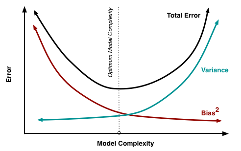
If we have a ton of classes, like say a neural network over a linear model, our $\mathcal{H}$ will be a large set, and thus we can’t get a tight bound. However, the optimal risk will also be hopefully lower.
Using a Neural Net:
We increase the complexity of our model, the set size becomes larger[increase risk], but the $inf R(f^*)$ is smaller[decrease risk]. Thus, using a neural net by itself won’t help much. Regularization saves the day here. It’s a way to control the complexity of our model[variance] while still decreasing risk. This situation is low bias, high variance.
Using a Linear Model:
We decrease the complexity of our model, the set size becomes smaller[decrease risk], but the $inf R(f^*)$ is larger[increase risk]. Thus, using a linear model can’t get us to the best solution. This situation is high bias, low variance.
BTW, this is one way of looking at bias-variance. I learned it by completely expanding the expected risk, so if you’re lost/looking for a more elegant solution, then wikipedia is for you, or check out my professor’s book:
Foundations of Machine Learning
What Next?
Although we have retrieved something concrete here, the resulting find is quite pessimistic for now. Why? Because this cannot be used for even linear models, let alone neural nets! The number of different hypotheses for linear models in $\Re^d$ space is not let alone finite, it’s not even countable! How can we ever hope to use uniform bound on such a large hypothesis class?
Enter VC Dimensions! They’ll be the main topic for next time, which, together with our grand equation, is the single most important theorem in learning theory.