Table of Contents

• Table of Contents
• $k$-armed Bandit Problem
• Action-value Methods
  • Estimating Action Values
  • Action Selection Rule : Greedy
  • Action Selection Rule : $\epsilon$-Greedy
  • Crux: Nonstationary Action Value
    • 1. Transience
    • 2. Convergence
  • Action Selection Rule: Optimistic Initial Values
  • Action Selection Rule: Upper-Confidence-Bound Selection
  • Gradient Bandit Algorithms
• Ending Remarks

To begin, we should note that bandit problems are a subset of tabular solution methods. The reason it’s called tabular is because we can fit all the possible states into a table. The tables tell us everything we need to know about the state of the problem, and so we can often find the exact solution to the problem that’s posed. We are following the book from Richard Sutton and Andrew Barto. ¹

$k$-armed Bandit Problem

One-armed bandit: a slot machine operated by pulling a long handle at the side.

We are faced with $k$ different actions. Each action gives you an amount of money, sampled from a distribution conditioned on the action. Each time step, you pick an action. You usually end with $T$ time steps. How do you maximize your gain?

For some time step $t$, we have an action, $A_t$, and a reward of the action, $R_t$. We denote the value* of an arbitrary action $a$ as $q_*(a)$:

\[q_*(a) = E[R_t|A_t = a]\]

What does this mean in english? It means “the value of an action $a$ is the expected value of the reward of that action(at any time).”

After reading that sentence 3-4 times, it makes sense right? If you knew that doing 1 action will give you the greatest expected value, then you abuse the hell out of it to max your gains.

Now we obviously want $q_*(a)$. It’s hard to get, though. $Q_t(a)$ is an estimate of $q_*(a)$ at time $t$. A desirable property is that:

\[lim_{t\to \infty}Q_t(a) = q_*(a)\]

So how do we make the $Q_t(a)$?

---

value*: in this case, it’s different than the concept of rewards. Value is the long run metric, meanwhile reward is the immediate metric. If you got hooked on heroin, it would be awesome rewards for the first hour, but it would be terrible value. Note here we wrote $q_*(a)$ as an expectation without sums of future rewards. This is not usually true in MDP’s, in which we will explore later, but as bandits is a stateless problem, we can use an abuse of notation here.

Action-value Methods

First, we have to estimate the action values, and then, we will decide what actions to do once we have estimates.

Estimating Action Values

One easy way to approximate $q_*(a)$ is to use sample means. What does this mean?

\[Q_t(a) = \frac{\sum_i^{t-1} R_i * 1_{A_i=a}}{\sum_i^{t-1} 1_{A_i=a}}\]

That might look loaded but really it’s just saying “for all the times we chose the action $a$, what was the average reward?” And this approximation of $q_*(a)$ is pretty good! Why? Because the expression above is literally SLLN(Strong Law of Large Numbers) in disguise.

What does that entail? It entails that $Q_t(a)$ converges almost surely to $q_*(a)$, or more formally:

\[P( lim_{t \to \infty}Q_t(a) = q_*(a)) = 1\]

This is stronger than a convergence in probability(which is already enough for most applications).

So this is great, asymptotically speaking we will definitely reach $q_*(a)$… right? (Not really, we will see why later)

Action Selection Rule : Greedy

The easiest and probably one of the worst thing you can do is to get addicted to heroin. That’s taking the greediest action, the one that gives you the greatest perceived value so far:

\[A_t = argmax_a Q_t(a)\]

We take whatever action has the greatest value so far. If we start as a blank slate, we’ll just keep taking the best value movement without exploring at all our other choices. This will easily lead to a suboptimal solution.

Action Selection Rule : $\epsilon$-Greedy

What could we do as an alternative? We can try something called an $\epsilon$-greedy method. This just means, for some small probability $\epsilon < 1$ at any time $t$, we choose from all actions uniformly, rather than greedily. It’s like tossing a coin, a random variable $X$, with $\epsilon$ probability of getting a tails, in which you would need to randomly select uniformly from all states. When you get heads, you would then perform the same greedy action.

Asymptotically speaking, we will take the actual optimal action with probability of more than $1-\epsilon$(once we found it, we’ll make sure to choose it all the time, but we also have $\frac{1}{\vert S\vert} * \epsilon$ chance to pick it in case of the uniform action choices).

Crux: Nonstationary Action Value

A lot of the time, our action values are changing with time. This is bad, because $q_*(a)$ is now dependent on time, so it’s more like $q_*(a,t)$.

Before, we had(we simplify the notation here):

\[Q_n = \frac{\sum_i R_i}{n-1}\]

Which can be expressed as:

\[Q_{n+1} = Q_n + \frac{1}{n}(R_n - Q_n)\]

Which is a very familiar update rule! Look like sgd by any chance?

Now this has the property of converging with probability 1 to $q_*(a)$ if it’s stationary. Now, what if it’s not? We definitely don’t want equal weighting of $R_0$ as $R_{n-1}$, because our most recent rewards reflect the current action values.

We can replace $\frac{1}{n}$ and replace it with $\alpha \in (0, 1]$:

\[Q_{n+1} = Q_n + \alpha(R_n - Q_n)\]

This is an exponential average, which geometrically decays the weight of previous rewards.

Now let’s abstract it even more: we introduce a function $\alpha_n(a)​$ which gives us the weight of a specific reward at time step $n​$ (in this case since we’re only concerned about an action, replace $\alpha_n(a)​$ with $\alpha_n​$):

\[Q_{n+1} = Q_n + \alpha_n(R_n - Q_n)\]

We need some properties about $\alpha_n(a)$ for this update to be arbitrarily convergent:

1. Transience

\[\sum_n \alpha_n(a) = \infty\]

implies that for any starting value $Q_1 \in \Re$, we can reach any arbitrary $q_*(a) \in \Re$.

2. Convergence

\[\sum_n \alpha_n(a)^2 < \infty\]

implies that the steps will be “small enough to assure convergence to a finite number”. I tried searching for a proof for #2, but it seemed like it required too much machinery. Like, 6 pages of machinery.

---

So why did we decide to set $\alpha_n(a) = \alpha \in (0,1]$? Isn’t that a constant? Wouldn’t we lose our guarantees for convergence?

Yes, we do. But it’s with good reason. We don’t want to converge to a specific value. The optimal action-value is nonstationary.

Action Selection Rule: Optimistic Initial Values

So far, we had to set initial values $Q_1(a)$ pretty arbitrarily. This is essentially a set of hyperparameters for initialization. One trick is to set the initial values for $Q_1(a) = C \forall a$, where $C > q_*(a) \forall a$.

This way, the learner’s estimate of $Q_n(a)$ will be decreasing at first, prioritizing exploration of all the states. Once the $Q_n(a)$’s have become close to $q_*(a)$, then greedy selection takes over.

One con is that this is not good for nonstationary problems. We are, in a way, doing simulated annealing and with enough time, we’re going to converge. We don’t want that!

Action Selection Rule: Upper-Confidence-Bound Selection

Remember this? I wrote this blog a while ago about bias variance tradeoff, with this as the holy grail result:

\[R(f) \leq [inf_{f^* \in \mathcal{H}}R(f^*)] + 2 \sqrt{\frac{log(\frac{2M}{\delta})}{2N}}\]

A quick recap of this is:

1. $R(f)$ is the (theoretical)risk of a hypothesis $f$.
2. $R(f*)$ is the minimum risk of a hypothesis $f$ in the space of hypothesis set $\mathcal{H}$.
3. $M$ is the size of our hypothesis set, $\vert \mathcal{H} \vert$.
4. $N$ is the number of samples.
5. $\delta$ is a constant. (If you have to know, it’s roughly the probability that a the hypothesis that we choose is bad)

What this is saying most importantly, is that:

1. At very low number of samples, our bound is very loose. We don’t know whether our current hypothesis is the best hypothesis.
2. The bigger our hypothesis set, the more loose our bound is for PAC learning.

Now, this transfers over to the reinforcement learning domain as well, in the form of Upper-Confidence-Bound action selection:

\[A_t = argmax_a Q_t(a)+c\sqrt{\frac{log(t)}{N_t(a)}}\]

Doesn’t this look familiar to the equality above? In here, some notations:

1. $N_t(a)$ is the number of times action $a$ has been selected for the $t$ time intervals.
2. $c$ is some constant we choose to control degree of exploration.

In the same analog, we can say that $t$ is the hypothesis space size $M$ from our previous equation. This is because as we increase on $t$, the sequence of actions $(a_n)$ up to $t$ grows in space. It is thus harder to select an $A_t$. However, as the amount of times we’ve selected $a$, $N_t(a)$ increases, we also gain information about how this action behaves.

UCB is a very powerful algorithm, and one can interpret it with a different view of the same problem: Greedy choosing vs. Regret minimization. In this case, we can interpret it as minimizing regret by giving enough exploration in all states before choosing the $argmax$, therefore “minimizing regret”.

Gradient Bandit Algorithms

We’ve been estimating $q_*(a)$, but what if I said there’s a different interpretation? How about we learn a preference for an action?

We’ll call the preference for the action $H_t(a)$. It’s not related to the reward at all, as we’ll see. We model $A_t$ as a gibbs distribution(in machine learning land, researchers call this the softmax distribution):

\[P(A_t = a) = \frac{e^{H_t(a)}}{\sum_b e^{H_t(b)}} = \pi_t(a)\]

Now we’re in business!

So how do we perform gradient-based MLE? So we do gradient ascent with respect to $H_t(a)$ because that’s what our variable is:

We want to maximize $E(R_t)$. Recall that:

\[q_*(a,t) = E(R_t|A_t = a)\] \[E(R_t) = \sum_a \pi_t(a)E(R_t|A_t=a) \quad{\text{(Total Expectation)}}\] \[E(R_t) = \sum_a \pi_t(a)q_*(a,t) \quad{\text{(By definition)}}\] \[\frac{\partial E(R_t)}{\partial H_t(b)} = \sum_a \frac{\partial \pi_t(a)}{\partial H_t(b)} q_*(a,t) \quad(q \text{ is independent})\]

So now that we have this, our general format for updates should be something like:

\[H_{t+1}(b) = H_t(b) + \frac{\partial E(R_t)}{\partial H_t(b)}\]

… for gradient ascent.

Now, let’s differentiate our gibbs distribution:

\[\begin{align*} &\frac{\partial \pi_t(a)}{\partial H_t(a)} = \\ &\frac{\partial (\frac{e^{H_t(a)}}{\sum_b e^{H_t(b)}})}{\partial H_t(a)} = \\ &\frac{e^{H_t(a)} * (\sum_b e^{H_t(b)} - e^{H_t(a)})}{(\sum_b e^{H_t(b)})^2} = \\ &\frac{e^{H_t(a)}}{\sum_b e^{H_t(b)}} * (1 - \frac{e^{H_t(a)}}{\sum_b e^{H_t(b)}}) = \\ & \pi_t(a) * (1-\pi_t(a)) \end{align*}\]

This is only one partial derivative of the whole gradient. What about the actions $b$ where $b \neq a$? I don’t really want to write out the $\LaTeX$ again, so here’s the answer:

\[\frac{\partial \pi_t(a)}{\partial H_t(b)} = -\pi_t(a)\pi_t(b) \forall b \neq a\]

We can thus observe a generalization:

\[\frac{\partial \pi_t(a)}{\partial H_t(b)} = \pi_t(a)(1_{a=b}-\pi_t(b)) \forall a,b\]

Okay, so now we can plug that into the equation:

\[\frac{\partial E(R_t)}{\partial H_t(b)} = \sum_a \frac{\partial \pi_t(a)}{\partial H_t(b)} q_*(a,t) = \sum_a \pi_t(a)(1_{a=b}-\pi_t(b)) q_*(a,t)\]

Now, we do some black magic. This is legal:

\[\sum_a \pi_t(a)(1_{a=b}-\pi_t(b)) q_*(a,t) = \sum_a \pi_t(a)(1_{a=b}-\pi_t(b)) (q_*(a,t) - X_t) \forall X_t \in \Re\]

Why is this true? Simply because:

\[\sum_a \pi_t(a)(1_{a=b}-\pi_t(b)) = \pi_t(a) - \sum_a\pi_t(a)\pi_t(b) = 0 \quad{\text{(total probability)}}\]

We’ll introduce one more weird addition:

\[\begin{align*} &\sum_a \frac{1}{\pi_t(a)}\pi_t(a)^2(1_{a=b}-\pi_t(b)) (q_*(a,t) - X_t) = \\ &E_a( (q_*(a,t) - X_t) * \pi_t(a)(1_{a=b}-\pi_t(b))/\pi_t(a))) = \\ &E_a( (q_*(a,t) - X_t) * (1_{a=b}-\pi_t(b))) \end{align*}\]

Because now, $q_*(a,t)$ is inside expectations of $a$, total expectations states that we can replace it with $R_t$.

One last thing is what do we choose for $X_t$? What is $X_t$? Well frankly, $X_t$ can be anything you want, but one can set this to the sampled average of previous rewards, $\bar{R}_t$, because then we would have an interpretable gradient. You don’t really need this to run the algorithm successfully, but this is chosen for stability, interpretability and historical reasons.

We’re all ready to see our new update rule!

\[H_{t+1}(b) = H_t(b) + E_a( (R_t - \bar{R_t} ) * (1_{a=b}-\pi_t(b)))\]

where $a$ is the action taken at time $t$.

Obviously, finding the expectation is hard, so we do a stochastic update and drop the expectations to get:

\[H_{t+1}(b) = H_t(b) + (R_t - \bar{R_t} ) * (1_{a=b}-\pi_t(b))\]

A simple way to choose the action is to pick $argmax_a \pi_t(a)$. So we’re done!

Ending Remarks

Here’s a plot of how these algorithms do compared to each other:

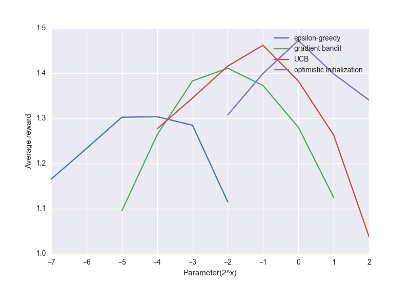
Although some of these methods are considered simple, it is not at all poorly performing. In fact, these are state of the art methods for many of reinforcement learning problems, and some of the ones we’ll learn later will be more complicated, more powerful, but more brittle.