Table of Contents

• Table of Contents
• Formalizations
  • The Agent-Environment Interface
  • Returns and Episodes
  • Policies and Value Functions
• Iterative Policy Evaluation
  • Proof of Convergence
• Policy Improvement
• Policy Iteration
• Value Iteration
  • Proof of Convergence
• See it in action!
  • Visual Results
• Conclusion

Previously, we discussed $k$-armed bandits, and algorithms to find the optimal action-value function $q_*(a)$.

Once we found $q_*(a)$, we could just choose $argmax_a q_*(a)$ all the time to reach the optimal solution.

We now go one more step further, and add a context to our reinforcement learning problem. Context in this case, means that we have a different optimal action-value function for every state:

This situation, where we have different states, and actions associated with the states to yield rewards, is called a Markov Decision Process(MDP).

We will be following the general structure of RL Sutton’s book¹, but adding extra proof, intuition, and a coding example at the end! I found some of his notation unnecessarily verbose, so some may be different.

Formalizations

The Agent-Environment Interface

We need to establish some notation and terminology here:

1. The decision maker is called the agent.
2. The decision maker’s interactions is with the environment, which give rewards.

For some time steps $t = 0,1,2,3,…$, we have associated with it, a state and an action $S_t \in \mathcal{S}, A_t \in \mathcal{A(s)}$. The reason actions is a function of state is we might have different permitted actions per state. If actions are the same in all states, then sometimes people abbreviate it as $\mathcal{A}$. With the associated action $A_t$, we receive a reward: $R_{t+1} \in \mathcal{R} \subset \Re$.

We thus have a sequence that looks like:

In a finite MDP:

$(R_t, S_t)_{t\geq 0}$ is a markov chain here. A markov chain, under discrete sigma algebra, is defined as:

Or in other words, $X_{n+1}$ , the future state, is dependent only on $X_{n}$, the present state. This is often called the markov property.

Thus, with the assumption, we can describe the entire dynamics of a finite MDP given:

We can marginalize $R_t$ and get:

which tells us the state-transition probabilities.

The expected reward for a state-action pair can be defined as:

Returns and Episodes

In general, if the agent has a finite lifespan, say $T$, then we want to maximize the reward sequence $G_t$:

Sometimes, $T$ can be a random variable.

However, many times our agent has an infinite lifespan, or we’re optimizing it to go to $\infty$(think of maximizing the time a robot is standing up). What do we do for that? We can re-formulate our problem using the idea of discounting:

This pretty much says, “the immediate rewards are better than the rewards later on, and the rewards way later on approaches 0”. And this discounting idea can apply to finite lifespan episodes as well, because we can have a final absorbing state $S_0$ where the rewards associated with any action in that state is 0.

Policies and Value Functions

We want to know how good it is to be in a specific state, and how good it is to take an action in a given state.

A policy is a mapping from states to probabilities of selecting an action. If an agent is following policy $\pi$, then he will take action $a$ at state $s$ with probability $\pi(a\vert s)$.

A value of a state $s$, under a policy $\pi$, is the expected return starting from $s$ if we take the policy’s suggested actions. It is denoted by $v_\pi(s)$, and is called a state-value function. We want our state-value function to be maximized at the end.

If we fix the action that we take at state $S_t = s$, then we would get an action-value function $q_\pi(s,a)$.

If you look closely, you can see a recursive equation in $v_\pi(s)$:

where the subscript $_p$ is for the probability distribution of $p(s’,r\vert s,a)$.

Do you see the recursion here? The expected value of $G_t$ is dependent on the expected value of $G_{t+1}$. This is also often called the Bellman equation for $v_\pi$. There is also a similar one for $q_\pi$, with similar expansions. This is obviously a hard equation to solve, and the result is the holy grail - $v_\pi$. How do we solve it? That’s the subject of a large part of reinforcement learning.

For interpretations sake, I’ll marginalize this a bit further and use definition of expectations:

To optimize for the action-value function for a specific state $s$, we need to change the parameter, which is $\pi$:

The above is the Bellman optimality equation. It’s pretty much saying: what’s the best possible value we can get out of a state?

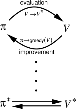
Iterative Policy Evaluation

I believe the notation in the book is quite verbose, so I will shorten it here for clarity. Recall our previous bellman equation:

We’ll denote $E_\pi(R\vert s)$ as $R_\pi(s)$ , and $E_\pi(R \vert s,a)$ as $R_\pi(s,a)$, etc. Then, we can vectorize our system of equations:

One way to solve this $V_\pi$ is to use an algorithm called iterative policy evaluation. It is the following update:

In vectorized form:

$V_{k+1} = R_\pi + \gamma P_\pi V_{k}$

with $v_0(s)$ being any arbitrary value in $\Re$.

Proof of Convergence

We can prove that $lim_{k \to \infty} v_k(s) \to v_\pi(s)$.

Proof:

Recall that $\gamma < 1$ for infinite time MDP’s, and that \(\vert \vert P_\pi\vert \vert=1 \forall \pi\), since this is a stochastic matrix.

By triangle inequality (of which, any proper norm exhibits):

Then we see that, ultimately:

Policy Improvement

Now that we have the true value function(or approaching), we want to find a better policy. For any existing policy $\pi$, we want to find a better $\pi’$, aka one that gives us $V_{\pi’} \succeq V_\pi$ .

So how do we find this $\pi’$? It’s actually pretty simple. If you know $v_\pi$, then why not just choose the action that gives you the greatest value on the next step? In formal terms:

Why is this better? It’s due to the idea that the max of the convex set is always greater than, or equal to the convex combination of any elements of the set. We essentially apply that simple idea here.

Well, let’s expand out what it means:

This means, if we take the action that gives us better results than our current $\pi$, at all $s$ at any time step, then we have created a new policy $\pi’$.

What happens when we reach equality of $\pi$ and $\pi’$?

Recall what the Bellman optimality equation says:

These two are exactly the same, implying that in the condition that equality occurs, we have reached the optimal policy.

Policy Iteration

So now that we have a way of evaluating $v_\pi(s)$, and a way to improve $\pi$, we can do something along the lines of:

1. Initialize with some arbitrary $\pi$, and arbitrary $v_\pi$ estimate.
2. Find the true $v_\pi$ for the $\pi$.
3. Find a better $\pi’$.
4. Repeat step 2 and 3 until $\pi’ = \pi$.

This is called the policy iteration algorithm. We have presented a possible method to solve MDP’s! We’re getting somewhere! Here’s a rough pseudocode:

def value_iter(V_prev):
    V_next = R + P * V_prev
    while V_next != V_prev:
        V_next = R + P * V_prev
    return V_next

def policy_improvement(prev_pi):
    for s in S:
    	pi(s) = prev_pi(s)
    for s in S:
    	pi(s) = argmax_a(q(s,a))
    return pi

def policy_iter(pi_prev):
    # Initialize
    q = find_q(pi_prev)
    V = find_V(pi_prev)
    pi_next = policy_improvement(pi_prev)

    # Policy Iteration
    while pi_next != pi_prev:
        pi_prev = pi_next
        q = find_q(pi_prev)
        V = find_V(pi_prev)
        pi_next = policy_improvement(pi_prev)
    return pi_next

Value Iteration

Recall policy iteration. Don’t you think it’s kind of slow to run the steps 2 and 3 together? Specifically, we’re going through all states in calculating the value function $v_\pi$, AND we’re going through all the states to calculate the next $\pi’$. This is a lot of work that we don’t need to do (roughly $O(N^2)$ run time).

Recall that $v_* = max_a q_{\pi_*}(s,a)$, and we’re trying to find $v_*$. Expanding it, $v_*$ is also equivalent to:

So this time, we run a different algorithm called value iteration:

This looks like some combination of policy evaluation and policy improvement in one sweep right?

So why does this converge, i.e. $\lim_{k \to \infty} v_k \to v_*$?

Proof of Convergence

We use the same contraction operator argument as before, but with a slight twist.

So:

As an aside, $\text{(1)}$ is true because:

So what does this algorithm look like?

def value_iter(prev_V):
    V = None
    while prev_V != V:
        V = prev_V
        for s in S:
            max_v_s = 0
            for a in A:
                # P(s,a) is a |S|x|A| matrix, where i,j=p(i,j|s,a)
                max_v_s = max(P(s,a) * (R(s,a) + gamma V[s]), max_v_s)
            V[s] = max_v_s
    return V # returns optimal V

After we get the optimal value, we can easily find the optimal policy.

See it in action!

To illustrate how this could work, we took the same situation in frozen lake, a classic MDP problem, and we tried solving it with value iteration. Here is the code below:

"""
Let's use Value Iteration to solve FrozenLake!

Setup
-----
We start off by defining our actions:
A = {move left, move right...} = {(0,1),(0,-1),...}
S = {(i,j) for 0 <= i,j < 4}
Reward for (3,3) = 1, and otherwise 0.
Probability distribution is a 4x(4x4) matrix of exactly the policy.
We have pi(a|s), where a in A, and s in S.

Problem formulation : https://gym.openai.com/envs/FrozenLake-v0/

Algorithm
---------
Because our situation is deterministic for now, we have the value iteration eq:

v <- 0 for all states.
v_{k+1}(s) = max_a (\sum_{s',r} p(s',r|s,a) (r + \gamma * v_k(s'))

... which decays to:

v_{k+1}(s = max_a (\sum_{s'} 1_(end(s')) + \gamma * v_k(s'))

Because of our deterministic state and the deterministic reward.
"""
N = 4
v = np.zeros((N, N), dtype=np.float32) # Is our value vector.
THRESHOLD = 1e-5
A = [(0,1),(0,-1),(1,0),(-1,0)]
MAP = [
    "SFFF",
    "FHFH",
    "FFFH",
    "HFFG"
]
def proj(n, minn, maxn):
    """
    projects n into the range [minn, maxn). 
    """
    return max(min(maxn-1, n), minn)

def move(s, tpl, stochasticity=0):
    """
    Set stochasticity to any number in [0,1].
    This is equivalent to "slipping on the ground"
    in FrozenLake.
    """
    if MAP[s[0]][s[1]] == 'H': # Go back to the start
        return (0,0)
    if np.random.random() < stochasticity:
        return random.choice(A)
    return (proj(s[0] + tpl[0], 0, N), proj(s[1] + tpl[1], 0, N))

def reward(s):
    return MAP[s[0]][s[1]] == 'G'
    
def run_with_value(v, gamma=0.9):
    old_v = v.copy()
    for i in range(N):
        for j in range(N):
            best_val = 0
            for a in A:
                new_s = move((i,j), a)
                best_val = max(best_val, reward(new_s) + gamma * old_v[new_s])
            v[i,j] = best_val
    return old_v

# Performing Value Iteration
plt.matshow(v)
old_v = run_with_value(v)
while norm(v - old_v) >= THRESHOLD:
    old_v = run_with_value(v)
plt.matshow(v)

# Extracting policy from v:
def pi(s, v):
    cur_best = float("-inf")
    cur_a = None
    for a in A:
        val = v[move(s, a)]
        if val > cur_best:
            cur_a = a
            cur_best = val
    return cur_a

# Plotting a nice arrow map.
action_map = np.array([
    [pi((i,j), v) for j in range(N)] for i in range(N)])
Fx = np.flip(np.array([ [col[1] for col in row] for row in action_map ]),0)
Fy = np.flip([ [-col[0] for col in row] for row in action_map ],0)
plt.quiver(Fx,Fy)

Visual Results

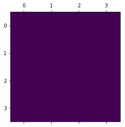
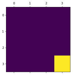
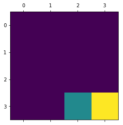
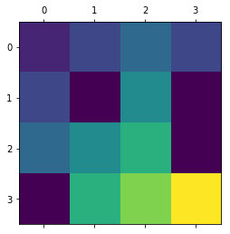
We plotted the colormap of value functions per state in our 2D world, and saw it converge to a reasonable policy:

Iteration 1:

Iteration 2:

Iteration 3:

Iteration 4:

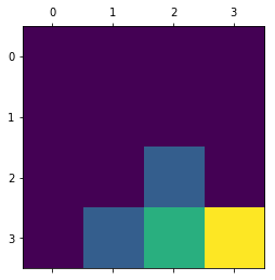
End Result:

In the end, our policy looks like:

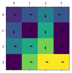
Pretty cool, huh? You can take a look at the code here.

Conclusion

So, our little exploration into MDP’s have been nice. We learned about how to formulate MDP’s and solve them using value iteration and policy iteration. We made a cool little coding example that we can use our algorithms to solve.

One major downside of these algorithms is that it’s not applicable for continuous-value domains. This means, for even a simple problem as Cart Pole, we won’t have a very smooth way of solving it(discretizing and running our algorithms might work, but it’s real hacky). We will explore ways to solve that issue next time!