Table of Contents

• Table of Contents
• Introduction
  • First-visit Monte Carlo
• Monte Carlo Action Values
• Monte Carlo Control
  • Exploring Starts
  • On-Policy: $\epsilon$-Greedy Policies
    • $\epsilon$-Greedy Convergence
  • Off-policy: Importance Sampling
    • Off-policy Notations
    • Ordinary Importance Sampling
    • Weighted Importance Sampling
    • Incremental Implementation
    • Extra: Discount-aware Importance Sampling
    • Extra: Per-reward Importance Sampling
• On-Policy Model in Python
  • Example: Blackjack
  • Example: Cliff Walking
• Conclusion

Previously, we discussed markov decision processes, and algorithms to find the optimal action-value function $q_*(s, a)$ and $v_*(s)$. We used policy iteration and value iteration to solve for the optimal policy.

It’s nice and all to have dynamic programming solutions to reinforcement learning, but it comes with many restrictions. For example, are there a lot of real world problems where you know the state transition probabilities? Can you arbitrarily start at any state at the beginning? Is your MDP finite?

Well, I think you’ll be glad to know that Monte Carlo methods, a classic way to approximate difficult probability distributions, can handle all of your worries associated with dynamic programming solutions!

Once again, we will be following the RL Sutton’s book¹, with extra explanation and examples that the book does not offer.

Introduction

Monte Carlo simulations are named after the gambling hot spot in Monaco, since chance and random outcomes are central to the modeling technique, much as they are to games like roulette, dice, and slot machines.

Monte Carlo methods look at the problem in a completely novel way compared to dynamic programming. It asks the question: How many samples do I need to take from our environment to discern a good policy from a bad policy?

This time, we’ll reintroduce the idea of returns, which is the long run expected gain:

Sometimes, if the episodes has a non-zero probability of lasting infinite time, then we will use a discounting factor:

We associate these returns $G_t$ with possible $A_t$’s to attempt to derive some kind of:

By the law of large numbers, as $N$ approaches $\infty$ we can get the exact expectation. We index over $i$ for the $i$-th simulation.

Now if this is an MDP(which 99% of reinforcement learning problems are), then we know it exhibits the Strong Markov Property which means:

With this, we can easily derive the fact that $t$ in the expectation is completely irrelevant, and we will be using $G_s$ from now on to denote the return starting from some state(move that state to $t = 0$).

First-visit Monte Carlo

A classic way to solve for the value function is to sample the return of the first occurence of $s$ , called first-visit MC prediction. Then a valid algorithm to find the optimal $V$ is:

pi = init_pi()
returns = defaultdict(list)
for i in range(NUM_ITER):
    episode = generate_episode(pi) # (1)
    G = np.zeros(|S|)
    prev_reward = 0
    for (state, reward) in reversed(episode):
        reward += GAMMA * prev_reward
        # backing up replaces s eventually,
        # so we get first-visit reward.
        G[s] = reward
        prev_reward = reward
    for state in STATES:
        returns[state].append(state)
V = { state : np.mean(ret) for state, ret in returns.items() }

Another method is called every-visit MC prediction, where you sample the return of every occurence of $s$ in every episode. The estimate converges quadratically in both cases to the expectation.

Monte Carlo Action Values

Sometimes, we don’t know the model of the environment, by that I mean what actions lead to what state, and how the environment in general interacts. In this case, we can use action values instead of state values, which means we solve for $q_*$.

We want to estimate $q_\pi(s,a)$, instead of $v_\pi(s)$. A simple change of G[s] to G[s,a] seems appropriate, and it is. One obvious issue is that now we went from $\mathcal{S}$ to $\mathcal{S} \times \mathcal{A}$ space, which is much larger, and we still need to sample this to find the expected return of each state action tuple.

Another issue is that as the search space increases, it becomes increasingly more likely that we might not be able to explore all state action pairs if we become greedy w.r.t our policy too quickly. We need to have a proper mix between exploration and exploitation. We will explain how we can overcome this problem in the next section.

Monte Carlo Control

Recall policy iteration from MDP’s. In this case, it’s not too different. We still fix our $\pi$, find $q_\pi$, and then find a new $\pi’$, and etc. The general process looks like:

We find the $q_{\pi_0}$’s in similar fashion to how we find our $v$’s above. We can improve our $\pi$’s by definition of the bellman optimality equation, and simply:

For more details on this, please refer to the previous MDP blog.

Now, the core crux of policy iteration in the context of monte carlo methods is, as we said, how do we ensure exploration vs. exploitation?

Exploring Starts

A way to remedy the large state space exploration is to specify that we start in a specific state and take a specific action, round robin style across all possibilities to sample their returns. This assumes that we can start at any state and take all possible actions at every start of an episode, which is not a reasonable assumption in many situations. However, for problems like BlackJack, this is totally reasonable, which means we can have an easy fix to our problem.

In code, we just need a quick patch to our previous code at (1):

# Before (Start at some arbitrary s_0, a_0)
episode = generate_episode(pi)
# After (Start at some specific s, a)
episode = generate_episode(pi, s, a) # loop through s, a at every iteration.

On-Policy: $\epsilon$-Greedy Policies

So what if we can’t assume that we can start at any arbitrary state and take arbitrary actions? Well, then we can still guarantee convergence as long as we’re not too greedy and explore all states infinitely many times, right?

The above is essentially one of the main properties of on-policy methods. An on-policy method tries to improve the policy that is currently running the trials, meanwhile an off-policy method tries to improve a different policy than the one running the trials.

Now with that said, we need to formalize “not too greedy”. One easy way to do this is to use what we learned in k-armed bandits - $\epsilon$-greedy methods! To recap, with $\epsilon$ probability we pick from a uniform distribution of all actions given the state, and with $1-\epsilon$ probability we pick the $argmax_a q(s,a)$ action.

Now we ask - does this converge to the optimal $\pi_*$ for Monte Carlo methods? The answer is it will converge, but not to that policy.

$\epsilon$-Greedy Convergence

We start off with $q$, and an $\epsilon$-greedy policy $\pi’(s)$.

Once again, we reach the statement that this $\epsilon$ greedy policy, like the greedy policy, performs monotonic improvements over $v_\pi$. If we back up on all time steps, then we get:

Which is what we wanted for convergence. $\blacksquare$

However, we need to find out what this policy can actually converge to. Obviously, since our policy is forced to be stochastic even if the optimal policy is deterministic, it’s not guaranteed to converge to $\pi*$. However, we can reframe our problem:

Suppose instead of having our policy hold the stochasticity of uniformly choosing actions with probability $\epsilon$, it is rather the environment that randomly picks an action regardless of what our policy dictates. Then, we can guarantee an optimal solution. The outline of the proof is to show that in $(1)$, if the equality holds then we have $\pi = \pi’$ and thus we have $v_\pi = v_{\pi’}$, and the equation is optimal under stochasticity due to the environment.

Off-policy: Importance Sampling

Off-policy Notations

Let’s introduce some new terms!

• $\pi$ is our target policy. We are trying to optimize this ones’ expected returns.
• $b$ is our behavioral policy. We are using $b$ to generate the data that $\pi$ will use later.
• $\pi(a\vert s) > 0 \implies b(a\vert s) > 0 \forall a\in \mathcal{A}$ . This is the notion of coverage.

Off-policy methods usually have two or more agents, one of which is generating the data that another agent tries to optimize upon. We call them behavior policy and target policy respectively. Off policy methods are “fancier” than on policy methods, like how neural nets are “fancier” than linear models. Similarly, off policy methods often are more powerful, with the cost of generating higher variance models and slower convergence.

Now, let’s talk about importance sampling.

Importance sampling answers the question: “Given $E_b[G]$, what is $E_\pi[G]$?”. In other words, how can you use the information you get from $b$’s sampling to determine the expected result from $\pi$?

One intuitive way you can think about it is: “If $b$ chooses $a$ a lot, and $\pi$ chooses $a$ a lot, then $b$’s behavior should be important to determine $\pi$’s behavior!”, and conversely: “If $b$ chooses $a$ a lot, and $\pi$ does not choose $a$ ever, then $b$’s behavior on $a$ should not have any importance towards $\pi$’s behavior on $a$.” Makes sense, right?

So that’s pretty much what importance-sampling ratio is. Given a trajectory ${(S_i, A_i)}_{i=t}^T$, the probability of this exact trajectory happening given policy $\pi$ is:

The ratio between $\pi$ and $b$ is simply:

Ordinary Importance Sampling

Now, there are many ways to utilize this $\rho_{t:T-1}$ to give us a good estimate of $E_\pi[G]$. The most rudimentary way is to use something called ordinary importance sampling. Suppose we had sampled $N$ episodes:

and denote the first arrival time of $s$ as:

and we wanted to estimate $v_\pi(s)$, then we can use empirical mean to estimate the value function using first-visit method:

Of course, this is easily generalizable to an every-visit method, but I wanted to present the simplest form to get the gist. What this is saying is we need to weigh the returns of each episode differently, because *the trajectories that are more likely to occur for $\pi$ should be weighted more than the ones that are never going to occur.

This method of importance sampling is an unbiased estimator, but it suffers from extreme variance problems. Suppose the importance ratio, $\rho_{\mathcal{T}(s):T^k-1}$ for some k-th episode is $1000$. That is huge, but can definitely happen. Does that mean the reward will necessarily be $1000$ times more? If we only have one episode, our estimate will be exactly that. In the long run, because we have a multiplicative relationship, the ratio may either explode or vanish. This is a little concerning for the purposes of estimation.

Weighted Importance Sampling

To reduce the variance, one easy, intuitive way is to reduce the magnitude of the estimate, by dividing by the total sum of all magnitudes of importance ratios(kind of like a softmax function):

This is called the weighted importance sampling. It is a biased estimate(with the bias asymptotically going to 0), but has reduced variance. Before, one could come up with a pathologically unbounded variance for the ordinary estimator, but each entry here has the maximum weight of 1, which bounds the variance by above. Sutton has suggested that, in practice, always use weighted importance sampling.

Incremental Implementation

As with many sampling techniques, we can implement it incrementally. Suppose we use the weighted importance sampling method from last section, then we can have some sampling algorithm of the form:

where $W_k$ could be our weight.

We want to form $V_{n+1}$ based off of $V_n$, which is very doable. Denote $C_n$ as $\sum_k^n W_k$, and we’ll keep this running sum updated as we go:

And $C_n$’s update rule is pretty obvious: $C_{n+1} = C_n + W_{n+1}$.

Now, this $V_n$ is our value function, but a very similar analog of this can also be applied to $Q_n$, which is our action value.

While we are updating the value function, we could also update our policy $\pi$. We can update our $\pi$ with the good old $argmax_a Q_\pi(s,a)$ .

Warning: Lots of math ahead. What we have right now is already good enough. This is approaching modern research topics.

Extra: Discount-aware Importance Sampling

So far, we have counted returns, and sampled returns to get our estimates. However, we neglected the internal structure of $G$. It really is just a sum of discounted rewards, and we have failed to incorporate that into our ratio $\rho$. Discount-aware importance sampling models $\gamma$ as a probability of termination. The probability of the episode terminating at some timestep $t$, thus must be of a geometric distribution $\sim geo(\gamma)$:

And full return can be considered an expectation over a random number of random variables $R_t$:

One can construct an arbitrary telescoping sum like so:

Inductively, we can see that for setting $k$ starting at $x$, we have $\gamma^x$.

We substitute this into $G$:

Which will lead to equivalent coefficients of $1$, $\gamma$, $\gamma^2$, etc on the $R_t$ terms. This means, now we can decompose $G_t$ into parts and apply discounting on the importance sampling ratios.

Now, recall that before we had:

If we expanded $G$, we would have, for one of these numerators in the sum:

Notice how we are applying the same ratio to all of the returns. Some of these returns, $G_{t:t+1}$, are being multiplied by the importance ratio of the entire trajectory, which is not “correct” under the modeling assumption that $\gamma$ is a probability of termination. Intuitively, we want $\rho_{t:t + 1}$ for $G_{t:t+1}$, and that’s easy enough:

Ah, much better! This way, each partial return will have their correct ratios. This combats the unbounded variance problem greatly.

Extra: Per-reward Importance Sampling

Another way to mitigate the problematic $\rho$ and its variance issues, we can decompose $G$ into its respective rewards and do some analysis. Let’s look into $\rho_{t:T-1}G_{t:T}$:

For each term, we have $\rho_{t:T-1}\gamma^kR_{t+k+1}$. Expanding $\rho$, we can see:

Taking the expectation without the constant $\gamma^k$:

Recall that you can only take $E(AB) = E(A)E(B)$ iff they are independent. It is obvious from the markov property that any $\pi(A_i\vert S_i)$ and $b(A_i\vert S_i)$ is independent of $R_{t+k+1}$ if $i \geq t+k+1$, and $\pi(A_i\vert S_i) \perp \pi(A_j\vert S_j) i \neq j$ (and same for $b$’s). We can take them out and get:

This may look extremely ugly, but one can observe that:

So we can really just completely ignore the second half:

What does this mean? We can really express our original sum in expectation:

Which will then, once again, decrease the variance of our estimator.

On-Policy Model in Python

Because Monte Carlo methods are generally in similar structure, I’ve made a discrete Monte Carlo model class in python that can be used to plug and play. One can also find the code here. It’s doctested.

"""
General purpose Monte Carlo model for training on-policy methods.
"""
from copy import deepcopy
import numpy as np

class FiniteMCModel:
    def __init__(self, state_space, action_space, gamma=1.0, epsilon=0.1):
        """MCModel takes in state_space and action_space (finite) 
        Arguments
        ---------
        
        state_space: int OR list[observation], where observation is any hashable type from env's obs.
        action_space: int OR list[action], where action is any hashable type from env's actions.
        gamma: float, discounting factor.
        epsilon: float, epsilon-greedy parameter.
        
        If the parameter is an int, then we generate a list, and otherwise we generate a dictionary.
        >>> m = FiniteMCModel(2,3,epsilon=0)
        >>> m.Q
        [[0, 0, 0], [0, 0, 0]]
        >>> m.Q[0][1] = 1
        >>> m.Q
        [[0, 1, 0], [0, 0, 0]]
        >>> m.pi(1, 0)
        1
        >>> m.pi(1, 1)
        0
        >>> d = m.generate_returns([(0,0,0), (0,1,1), (1,0,1)])
        >>> assert(d == {(1, 0): 1, (0, 1): 2, (0, 0): 2})
        >>> m.choose_action(m.pi, 1)
        0
        """
        self.gamma = gamma
        self.epsilon = epsilon
        self.Q = None
        if isinstance(action_space, int):
            self.action_space = np.arange(action_space)
            actions = [0]*action_space
            # Action representation
            self._act_rep = "list"
        else:
            self.action_space = action_space
            actions = {k:0 for k in action_space}
            self._act_rep = "dict"
        if isinstance(state_space, int):
            self.state_space = np.arange(state_space)
            self.Q = [deepcopy(actions) for _ in range(state_space)]
        else:
            self.state_space = state_space
            self.Q = {k:deepcopy(actions) for k in state_space}
            
        # Frequency of state/action.
        self.Ql = deepcopy(self.Q)

        
    def pi(self, action, state):
        """pi(a,s,A,V) := pi(a|s)
        We take the argmax_a of Q(s,a).
        q[s] = [q(s,0), q(s,1), ...]
        """
        if self._act_rep == "list":
            if action == np.argmax(self.Q[state]):
                return 1
            return 0
        elif self._act_rep == "dict":
            if action == max(self.Q[state], key=self.Q[state].get):
                return 1
            return 0
    
    
    def b(self, action, state):
        """b(a,s,A) := b(a|s) 
        Sometimes you can only use a subset of the action space
        given the state.

        Randomly selects an action from a uniform distribution.
        """
        return self.epsilon/len(self.action_space) + (1-self.epsilon) * self.pi(action, state)

    
    def generate_returns(self, ep):
        """Backup on returns per time period in an epoch
        Arguments
        ---------
        
        ep: [(observation, action, reward)], an episode trajectory in chronological order.
        """
        G = {} # return on state
        C = 0 # cumulative reward
        for tpl in reversed(ep):
            observation, action, reward = tpl
            G[(observation, action)] = C = reward + self.gamma*C
        return G
    
    
    def choose_action(self, policy, state):
        """Uses specified policy to select an action randomly given the state.
        Arguments
        ---------
        
        policy: function, can be self.pi, or self.b, or another custom policy.
        state: observation of the environment.
        """
        probs = [policy(a, state) for a in self.action_space]
        return np.random.choice(self.action_space, p=probs)

    
    def update_Q(self, ep):
        """Performs a action-value update.
        Arguments
        ---------
        
        ep: [(observation, action, reward)], an episode trajectory in chronological order.
        """
        # Generate returns, return ratio
        G = self.generate_returns(ep)
        for s in G:
            state, action = s
            q = self.Q[state][action]
            self.Ql[state][action] += 1
            N = self.Ql[state][action]
            self.Q[state][action] = q * N/(N+1) + G[s]/(N+1)
    
    def score(self, env, policy, n_samples=1000):
        """Evaluates a specific policy with regards to the env.
        Arguments
        ---------
        
        env: an openai gym env, or anything that follows the api.
        policy: a function, could be self.pi, self.b, etc.
        """
        rewards = []
        for _ in range(n_samples):
            observation = env.reset()
            cum_rewards = 0
            while True:
                action = self.choose_action(policy, observation)
                observation, reward, done, _ = env.step(action)
                cum_rewards += reward
                if done:
                    rewards.append(cum_rewards)
                    break
        return np.mean(rewards)
    
if __name__ == "__main__":
    import doctest
    doctest.testmod()

Try it out for yourself if you would like to use it in different gyms.

Example: Blackjack

We use OpenAI’s gym in this example. In here, we use a decaying $\epsilon$-greedy policy to solve Blackjack:

import gym
env = gym.make("Blackjack-v0")

# The typical imports
import gym
import numpy as np
import matplotlib.pyplot as plt
from mc import FiniteMCModel as MC

eps = 1000000
S = [(x, y, z) for x in range(4,22) for y in range(1,11) for z in [True,False]]
A = 2
m = MC(S, A, epsilon=1)
for i in range(1, eps+1):
    ep = []
    observation = env.reset()
    while True:
        # Choosing behavior policy
        action = m.choose_action(m.b, observation)

        # Run simulation
        next_observation, reward, done, _ = env.step(action)
        ep.append((observation, action, reward))
        observation = next_observation
        if done:
            break

    m.update_Q(ep)
    # Decaying epsilon, reach optimal policy
    m.epsilon = max((eps-i)/eps, 0.1)

print("Final expected returns : {}".format(m.score(env, m.pi, n_samples=10000)))

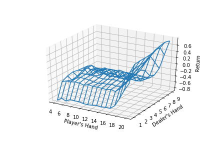
# plot a 3D wireframe like in the example mplot3d/wire3d_demo
X = np.arange(4, 21)
Y = np.arange(1, 10)
Z = np.array([np.array([m.Q[(x, y, False)][0] for x in X]) for y in Y])
X, Y = np.meshgrid(X, Y)

from mpl_toolkits.mplot3d.axes3d import Axes3D

fig = plt.figure()
ax = fig.add_subplot(111, projection='3d')
ax.plot_wireframe(X, Y, Z, rstride=1, cstride=1)
ax.set_xlabel("Player's Hand")
ax.set_ylabel("Dealer's Hand")
ax.set_zlabel("Return")
plt.savefig("blackjackpolicy.png")
plt.show()

And we get a pretty nice looking plot for when there is no usable ace(hence the False in Z for meshgrid plotting).

I also wrote up a quick off-policy version of the model that’s not yet polished, since I wanted to just get a benchmark of performance out. Here is the result:

Iterations: 100/1k/10k/100k/1million.
Tested on 10k samples for expected returns.

On-policy : greedy
-0.1636
-0.1063
-0.0648
-0.0458
-0.0312

On-policy : eps-greedy with eps=0.3
-0.2152
-0.1774
-0.1248
-0.1268
-0.1148

Off-policy weighted importance sampling:
-0.2393
-0.1347
-0.1176
-0.0813
-0.072

So it seems that off-policy importance sampling may be harder to converge, but does better than the epsilon greedy policy eventually.

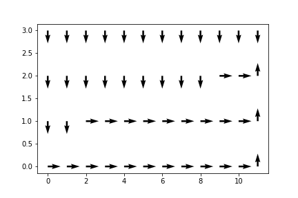
Example: Cliff Walking

The change to the code is actually very small because, as I said, Monte Carlo sampling is pretty environment agnostic. We changed this portion of the code(minus the plotting part):

# Before: Blackjack-v0
env = gym.make("CliffWalking-v0")
# Before: [(x, y, z) for x in range(4,22) for y in range(1,11) for z in [True,False]]
S = 4*12 
# Before: 2
A = 4 

And so we ran the gym and got -17.0 as the $E_\pi(G)$. Not bad! The cliff walking problem is a map where some blocks are cliffs and others are platforms. You get -1 reward for every step on a platform, and -100 reward for every time you fall down the cliff. When you land on a cliff, you go back to the beginning. For how big the map is, -17.0 per episode is a near-optimal policy.

Conclusion

Monte Carlo methods are surprisingly good techniques for calculating optimal value functions and action values for arbitrary tasks with “weird” probability distributions for action or observation spaces. We will consider better variations of Monte Carlo methods in the future, but this is a great building block for foundational knowledge in reinforcement learning.